How to make a linkage map
Linkage maps are constructed on the basis of analysis of many segregating markers in a large segregating population. The three main steps that lead to the development of a linkage map are as follows:
(1) Development of a mapping population
(2) Genotyping: identification of polymorphism of markers in parents and progeny and running the markers
(3) Linkage analysis of markers: determining the degrees of associated segregation between markers (and possibly between markers and a gene for a trait) and construction of a genetic linkage map
After the linkage map has been constructed, these steps can be followed by:
(4) Phenotyping: scoring phenotypic traits in a mapping population, needed to later find associations of markers to phenotypic traits in a QTL analysis or in a linkage analysis of a qualitative monogenic trait (see 3)
(5) QTL analysis: establishing which regions in the genome are associated with a quantitative phenotypic trait
Ideally, once the linkage map is available, this map gives valuable knowledge of markers and their position on the genome. Such information can be used to locate genes in the original mapping population. But other segregating plant material (e.g. progeny of a cross of different parents) may also be genotyped with these markers, to find associations with some traits of interest. If such an association is found, we may conclude from the known position of the marker on the linkage map, that in that other material the gene for the associated trait should be in the same chromosome region. However, many markers used to create the map, might not be polymorphic in the other population. Also, the trait of interest might be influenced by different genes in different populations, because some genes might be polymorphic in the mapping population and not polymorphic in the new population and vice versa. This will be explained in further detail later on.
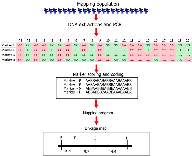
Steps involved in the construction of a linkage map with DNA markers.
(1) Development of a mapping population: this example is based on a small recombinant inbred population (RIL) from a cross, consisting of only 20 RIL individuals. Note that this low number of individuals is not realistic. In the real world, the mapping population should be large (a large number of RILs in this case): in small populations linkage between markers and markers and associations between markers and a trait cannot be established with any reliability.
(2) Genotyping: DNA extraction and PCR, followed by:
Identification of polymorphisms and running the markers: the first parent (P1) is scored as an 'A' whereas the second parent (P2) is scored as a 'B' for each marker; each individual is scored likewise. In this case 'A' refers to the homozygous diploid genotype of an individual equal to the parent P1 genotype (e.g. MM), and 'B' to the homozygous diploid genotype of an individual equal to that of parent P2 (e.g. mm).
(3) Linkage analysis: estimation of recombination frequencies of all marker pairs and sometimes of genes for qualitative traits. Determine which markers and genes are linked, and constuct a genetic linkage map by assignin
g markers to linkage groups, establishing marker order, and genetic distances in cM units per linkage group.
After the linkage map has been constructed, these steps are followed by:
(4) Phenotyping: Scoring of phenotypic traits in a mapping population,needed to later find associations of markers to phenotypic traits in a QTL analysis or in a linkage analysis of a qualitative monogenic trait (see 3)
(5) QTL analysis: establishing which regions in the genome are associated with a quantitative phenotypic trait