Linkage analysis in practice
For a few markers, linkage analysis can in some cases be performed manually, but for large numbers of markers, or situations with dominant markers or varying numbers of missing values, computer programs are needed. Commonly used software programs for construction of a linkage map include Mapmaker and JoinMap. These programs calculate/estimate all pairwise recombination frequencies between markers and determine the significance of linkage or of 'association'. The evidence of linkage is often quantified in a LOD score: the Logarithm Of Odds, which is the ten-based logarithm of the ratio of the likelihood of the observed genotype frequencies under linkage versus the likelihood in case the markers would be unlinked.

Usually, to construct linkage maps, the threshold value for the LOD value of two markers to be linked is set to a value between 3 and 4 (LOD threshold for linkage). This threshold can be defined by the user of the software or it can be indicated by the computer program, or the effect of different thresholds could be compared. A LOD threshold of 3 means that linkage between two markers, given the genotype frequencies, is 1000 times more likely than if markers were unlinked (3 is the 10log of 1000). A lower LOD threshold corresponds to detecting linkages under a relatively low significance level, whereas a higher LOD threshold would be more stringent: they tend to lead to decisions that markers that seem loosely associated are unlinked. However, the LOD threshold of 3 corresponds to a confidence level of about 95%. About 5% of the indicated linkages may be actually false positives: some of the (slightly) associated markers only are associated by chance and not by true linkage. This can be very undesirable since it might result in joining linkage groups that in reality correspond to different chromosomes. Also markers might be assigned to linkage groups based on not accurate enough information, for example if they show distorted segregation, had poor signals on the gel, or were entered with some trivial errors.
|
|
Hypothetical linkage map, consisting of five linkage groups (each probably representing a chromosome) and 26 markers. This picture represents an ideal situation, where markers are more or less evenly spaced. In a real situation, this is almost never the case, but we will observe gaps and clusters (see next example). The figures give the percentage of recombination between adjacent loci that is observed in this mapping population.
|
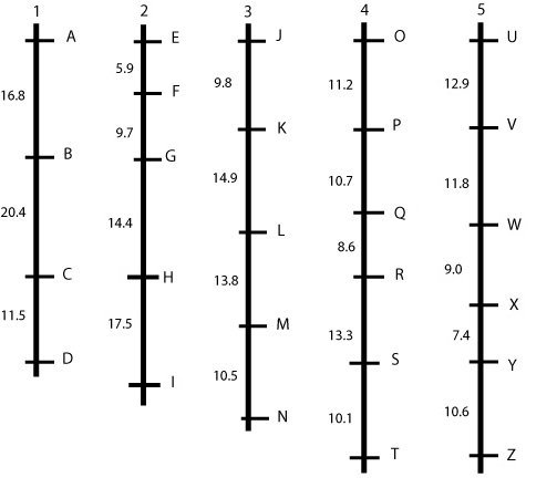
An ideal but unrealistic linkage map is shown in the figure above: linked markers are about evenly spaced and grouped together into 'linkage groups,' which, in an ideal situation, represent entire chromosomes or parts of chromosomes. Mostly, we prefer a linkage map with "spaces" of at most 5 cM between loci, so this map is not yet sufficiently "saturated".
In case we find large gaps, we should try to find more polymorphic markers between the parents and run those markers, hoping that some of them will map in the middle of some of the largest gaps.
Linkage maps may (at some chromosome regions) be more dense than necessary for mapping genes. This may be the case where thousands of markers were mapped, or in places where marker loci clustered, i.e. many markers map to almost the same locus (see for example in the middle of chromosome 3 in the figure below). We may, for further application of the map, delete most markers from the data set, and only retain the most reliably scored ones (with fewest missing data), with intervals of about 5 cM. Such a map is called "skeletal linkage map". This helps to reduce computational time for some calculations involved in map construction.
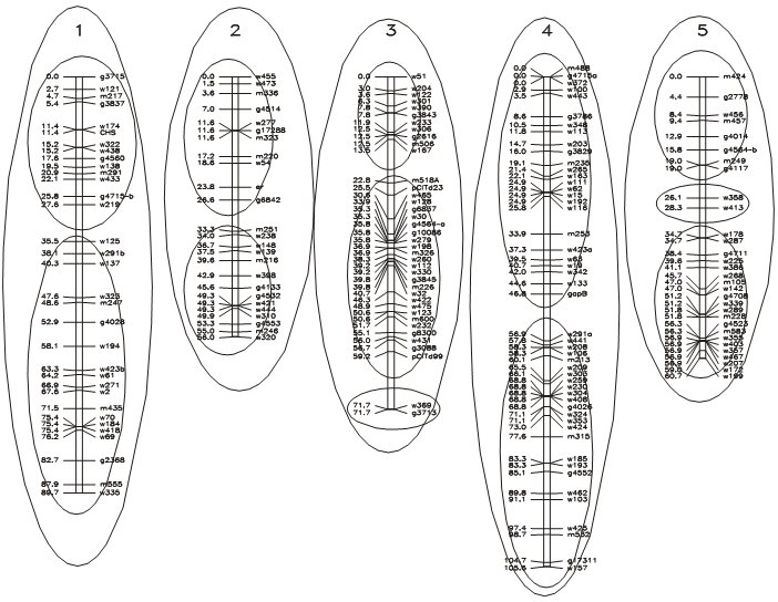
Assignment of markers to linkage groups at LOD = 12.0 (inner circles) and LOD = 5.9 (outer circles). (Maps calculated according to the (correct) assignment of 5 linkage groups, presumably located on 5 chromosomes).
Data source: Lister & Dean, Arabidopsis thaliana. Picture source: P. Stam, Study guide for the Wageningen MSc. course 'Modern statistics for the life sciences'.
The figure above shows a real-life situation of the assignment of markers to linkage groups, including clusters and gaps. Notice that a stringent (high) LOD threshold leads to more linkage groups than the haploid chromosome number.
When constructing a linkage map from scratch (with a set of markers that have not previously been assigned to linkage groups or chromosomes) it is recommended to stay 'at the safe side' by using a relatively high LOD threshold. This will prevent that groups of markers that in reality are on different chromosomes are incorrectly assigned to the same linkage group. Anchor markers known from other data sets may help to correctly group different linkage groups.
In the end, the number of linkage groups should be the same as the number of chromosome pairs in the organism's diploid genome (for autogamous crops; for cross pollinated crops often maps per parent are made, so there it could be twice the number of haploid chromosomes; for polyploids it could again be different, depending on the level of integration; e.g. for a tetraploid it could be either 1 linkage group per chromosome, 2, or 8). Assigning chromosome numbers to the linkage groups is done on the basis of (historical) knowledge on the location of certain morphological markers, resistance genes and standard markers mapped in other studies on the same organisms, and that are included in the present study as well, or, for sequenced crops, based on sequence information of these markers on the chromosomes.
Summary
→ A LOD score quantifies the strength of evidence of linkage (or sometimes of dependence) between markers based on genotype frequencies observed in the mapping population
→ The LOD threshold is a threshold above which genes/markers are considered linked