Linkage mapping

Step 2. Genotyping: identification of polymorphisms, development of markers, and scoring in a mapping population

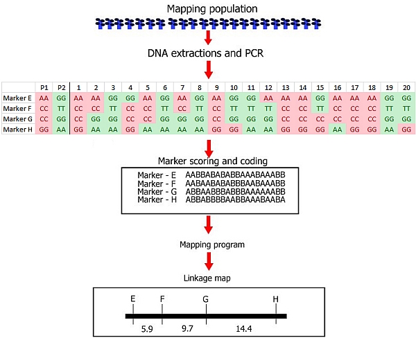
As we have seen before, the three main steps of linkage map construction are:

(1) Development of a mapping population

(2) Genotyping: identification of polymorphism of markers in parents and progeny and running the markers.

(3) Linkage analysis of markers: determining the degrees of associated segregation between markers and construction of the linkage map

After the linkage map has been constructed, these steps are followed by:

(4) Phenotyping: collect trait values for QTL analysis or mapping of a qualitative trait

(5) QTL analysis

 

Polymorphic markers

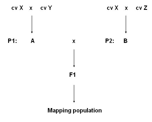
The second step in the construction of a linkage map is to identify DNA markers that reveal differences between alleles (i.e. polymorphic markers), and run them on the members of the mapping population. This running of markers on a mapping population is called genotyping. It is critical that sufficient polymorphism already exists. For mapping populations derived from homozygous parents, these parents are usually chosen on the basis of a clear contrast in the trait of interest and on a high expected level of polymorphism over the genome. Usually any pair of cultivars shows polymorphism. However, in some crops, e.g. tomato, genotypic uniformity is very high, and lack of polymorphism may be a problem. Generally, the less related (for example if collected on different continents) the higher the genetic variability and hence the degree of polymorphism. When there is no polymorphism, no linkage map can be made. If two parents share one of their ancestors, some parts of their genome may be not polymorphic.

Once polymorphic markers have been identified, they must be screened across the entire mapping population, including the parents. This is known as marker genotyping of the population. 

DNA sampling and genotyping

Before markers can be scored, DNA must be extracted from each individual of the mapping population and from the parents. There are several DNA isolation techniques. Since usually large numbers of plants should be sampled, a quick method is desirable. Such quick methods are available, but they tend to give a bit less reliable patterns when processed to reveal markers. More laborious methods may give a more stable and reliable marker pattern, and the DNA may be stored longer. For markers that are based on Southern Blotting (RFLP) much larger amounts of DNA need to be sampled than for markers that depend on PCR amplification. That is one of several reasons why RFLP markers became obsolete.

Errors

Recording should be done very carefully: errors are a very common and disturbing factor in map construction. Sources of errors include unclear signals on the gel or blot, and simple typing errors in the spreadsheet. In case of a doubtful signal on the gel, it is better to enter a missing value symbol in the data sheet. The reason for this is that genotyping errors will often count as extra recombinants in the data analysis, and often even as 'double recombinants' (both to the left side and to the right side of an incorrectly scored marker, a false 'recombination' is observed). Errors in genotyping increase the length of genetic maps, cause incorrect ordering and distance estimation among markers and reduce the power of gene detection and QTL analysis and decrease the accuracy of the results, for example of the estimated effects of genes or QTLs on a phenotypic trait 

Examples

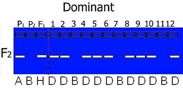
Examples of DNA markers screened across different populations are shown in the figure below.

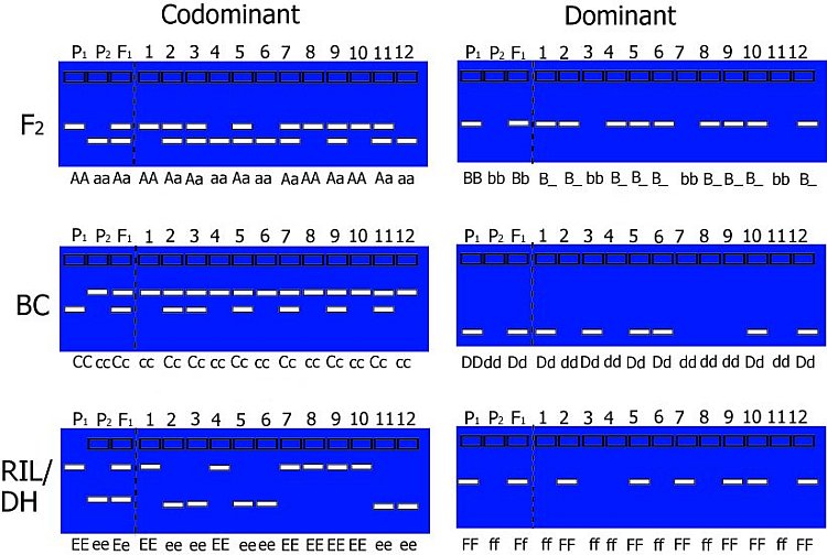
Hypothetical gel photos representing segregating codominant markers (left) and dominant markers (right) for typical mapping populations. Codominant markers reveal the complete genotype for a marker. Note that dominant markers cannot discriminate between heterozygotes and one homozygote genotype in F2 populations. 

The expected segregation ratios for codominant and dominant markers are presented in the table. Significant deviations from expected ratios can be analysed using chi-square tests. Generally, markers will segregate in a Mendelian fashion.

Sometimes, distorted segregation ratios may be encountered so that we cannot always assume nice 1:1, 1:2:1 or 3:1 segregations in a progeny. Be aware that deviations from these expected segregation ratios might be caused by scoring difficulties or quality issues (bad quality DNA, for example) but also by biological phenomena (gametophytic or zygotic selection, self-incompatibility, or deleterious loci). However, scoring difficulties and quality issues would usually be observed at individual loci, while neighbouring markers are unaffected, whereas biological phenomena would usually affect a number of markers in the same genomic region.

 

Note: larger numbers of markers are usually indicated with M1, M2, M3 etc., also to avoid confusion with the coding explained in the next paragraph.

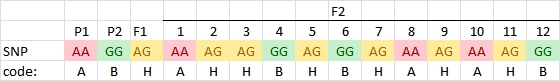
Coding (in JoinMap and MapQTL)

In the examples above we have given the allele names of the markers, e.g. AA, Aa and aa, and BB, Bb, B_ and bb, but in the case of progenies from homozygous parents, for large numbers of markers a special type of coding is used:

• A genotype with both alleles contributed by Parent 1 is coded A (=homozygous as parent 1)
• A genotype with both alleles contributed by Parent 2 is coded B (=homozygous as parent 2)
• A genotype with one allele from either parent (for example F₁) is coded H (heterozygote):

However, in the case of a dominant marker in an F₂ population, we cannot tell if an individual is heterozygous or homozygous for the dominant marker allele. We only know that it is not homozygous for the null allele. In those cases we need more codes:

• If an individual could carry the same alleles as Parent 2 OR the F₁, but not Parent 1 it is coded C (indicating that it might be B or H, but not A):

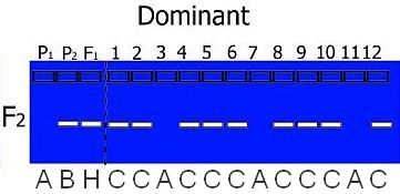
• If an individual could carry the same alleles as Parent 1 OR the F₁, but not Parent 2 it is coded D (indicating that it might be A or H, but not B):

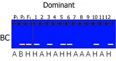
Coding is dependent on the type of mapping population used. For example, in a RIL or DH population only homozygotes are present (so codes H, C or D do not appear in the offspring) and in a BC population, we know that heterozygotes are present and only one type of homozygote: the one from the parent used for backcrossing:

In practice, you also may have missing data or bands that are unclear. These receive a special code U.

Coding in F1 progenies of crosses of heterozygous parents of an allogamous crop is different, and even different for different markers, since different segregation types may be present at the same time: for some markers P1 will be heterozygous and P2 homozygous; for other markers P1 may be homozygous and P2 heterozygous, while for again other markers P1 and P2 may both be heterozygous for the same alleles or for different alleles. In polyploid crosses the coding is again different because dosage differences need to be taken into account as well as heterozygosity/homozygosity, but this will not be treated here.

Even though it is, by far, preferred that the parents of a mapping population are also genotyped for all the markers, map construction is still possible if one or both parents are missing. The coding then has to be adapted to reflect this uncertainty.

 

Summary

→    To identify and score polymorphic DNA markers, DNA must be extracted from each individual plant in the mapping population and the parents

→    Segregation of markers generally follows a Mendelian fashion, but distorted segregation is not uncommon

→    Codes used for genotyping as used in mapping programs such as JoinMap and MapQTL are listed in the table above

 

I want extra information | Move on to: Step 3. Linkage analysis of markers