Source: Wikipedia.
Linkage mapping
Marker-assisted selection
The traits of a plant (i.e. the outer and inner appearance and performance) are called the phenotype. The phenotype of a plant is determined both by genetic factors (genotype) and non-genetic factors ("environment"). It is the challenge for the plant breeder to determine the genetic component of the phenotype, since that is the aspect that can be improved by selection. The genotype of a plant is encoded in DNA, especially in elements that are called "genes". Most genes exist in various forms (alleles), each with a slightly different DNA sequence and each with a potentially different effect on the plant (or occasionally: total absence of the allele, or presence of a non-functional mutant allele). A breeder is interested in accumulating favorable alleles in his germplasm, and discard as much as possible unfavorable alleles. This selection can be done by evaluating the traits, but it would be in many cases efficient to select directly on the basis of the DNA sequence of the most favorable alleles, especially for traits that are hard or expensive to judge or quantify.
|
|
|
Source: Wikipedia. |
Two kinds of traits exist:
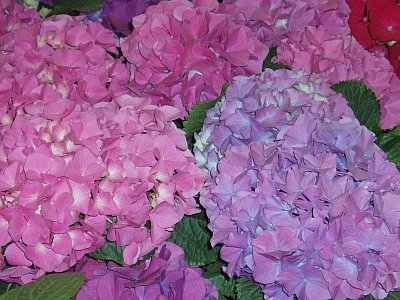
1. qualitative traits (simple discrete traits), such as smooth or wrinkled seeds or flower color. These traits are controlled by single (or few) genes and are typically not much influenced by the environment. (Beware that often exceptions exist, like e.g. blue and pink flower color depending on the soil pH in Hydrangea macrophylla). For qualitative traits, the individuals in a population can be assigned to different classes based on their phenotype, and these classes correspond very closely to different genotypes at the relevant locus/loci. Not necessarily all genotypes can be distinguished by the phenotype, as for example in the case of dominance, where the heterozygote has the same phenotype as one of the homozygotes, but the class containing the 'dominant' phenotype (combining the heterozygote and the homozygote for the dominant allele) can still be distinguished from the other homozygous class, the phenotype that corresponds to the homozygote for the recessive allele.
2. quantitative traits, such as yield, height, or quality. Such quantitative traits are strongly influenced by the environment, and they are usually controlled by several to many genes, and some of these may have a small effect on the trait. For quantitative traits there is no direct correspondence in discrete classes between the observed phenotype and the underlying genotypic differences. In selection programmes these traits are often measured on some quantitative scale (in cm or kg for example). The chromosomal region in which one or more genes that affect a quantitative trait are located is called a quantitative trait locus (QTL; plural: quantitative trait loci, QTLs). QTLs are regions on the genome that have a statistical association with a quantitative trait. A QTL may comprise one or more functional genes; QTLs are not the genes themselves. QTL analysis will be treated later in this module.
More information can be obtained through this nice, old-fashioned style, video on dominant and recessive genes. Note that in that video tallness is presented as a qualitative trait, rather than a quantitative trait! This may happen if the plant length is determined by one strong-effect gene. Tallness can be measured on a quantitative scale (cm), but in this particular example it can also be scored in two discrete classes: tall and short. In most cases, however, the inheritance of plant height is determined by several genes, each with a relatively small contribution. They require QTL mapping procedures to be discovered (this will be treated in the next chapter).
Summary
→ Qualitative traits are controlled by single or few genes with clear effects on the phenotype
→ Quantitative traits are controlled by multiple genes, some of which may have relatively small effects, and in addition these traits are influenced very much by environmental conditions
→ A QTL is a chromosomal region showing a statistical association with a quantitative trait, which is ascribed to the presence of one or more genes influencing the trait
I want an alternative explanation | Move on to: Linkage
The phenotype of a plant describes what a plant looks like: all its traits. Examples of traits are its color, its length, its leaf shape etc. Also its inner appearance, such as disease resistance, sugar content, or types of proteins and fibers formed are part of the phenotype.
The genotype of a plant is all the information present in its DNA. Some parts of the DNA are genes: they are transcribed and code for proteins that play a role in the physiology and performance of the plant. Genes have effect through the processes of transcription and translation. Some other parts of the DNA do not code for proteins and are called non-coding areas. Both genes and non-coding areas make up the genotype.
The environment greatly influences the appearance and performance of the plant. A plant receiving sufficient light and nutrients AND containing many genes that positively affect growth will probably result in a plant with a high biomass.
Qualitative traits are discrete traits that have two or several character values in clearly distinct discrete classes (like eye color in humans). They are often controlled by a single gene with a major effect, or few genes with large effects and they are not much influenced by non-genetic factors like the environmental conditions. A specific gene has a specific place on a specific chromosome, called a locus. Since the effect of the gene is so large, typically a breeder can conclude from the phenotype of each plant whether it carries the one or the other allele of the gene, so the genotype is readily deduced from the phenotype (although not every genotype may be a distinct class, as in the case of dominant genes). However, as we will see later, it still may be very efficient to select on the basis of molecular markers rather than on the basis of phenotype.
A well-known example of a qualitative trait in plant breeding is seed coat of peas. In the nineteenth century, Gregor Mendel discovered that the traits 'smooth' or 'wrinkled' seed coats of peas were inherited from the parents and that these traits were controlled by two 'factors': two alleles of one gene. He formulated the basic 'Laws of heredity'. Mendel's first law of equal segregation comes down to saying that heridatory factors (now called: genes) in an individual appear in pairs (now called: alleles) of which two variants segregate into equal proportions in the egg cells or in the sperm/pollen cells. At fertilization these fuse at random to produce progeny individuals, giving rise to recognizable mathematical ratios, in the progeny population, such as 1:1, 1:2:1 (in case of codominant genes) or 3:1 (for dominant genes in an F2) for the different variants, as was the case for smooth/wrinkled seed coat of peas.
Quantitative traits, such as yield or plant height, often (but not always) have a continuous distribution. The variation in the values of the trait is usually influenced by multiple genes. and, in addition, to quite some extent also by non-genetic factors, environmental conditions. Each of the genes involved may therefore contribute only a relatively small part to the total phenotypic variation, but some large-effect genes may also be present. The exact location and identity of the contributing genes is often unknown but an association between the trait values and variation in a certain region on the genome can be discovered by statistical tests. Such a region is called a quantitative trait locus (QTL) and the discovery of QTLs is called QTL analysis. QTLs are loci (or regions, and hence, no genes by themselves!) on the genome that have a statistical association with a quantitative trait. Here the application of markers will be necessary, in research but also for a plant breeder to determine which of the plants have desirable alleles and which ones have undesirable alleles influencing the trait. A reported QTL could indicate that there is a gene or that there are multiple genes present in the region that influence the trait. However, as in any statistical analysis, false positives are also possible: detected associations that are not corresponding to actual genetic differences.
Show/hide comprehension question...
When two genes (or a gene and a marker, or two markers) are situated closely together on a chromosome, they often inherit together: their loci are linked. Diploid organisms have two sets of chromosomes: one set from the father and one set from the mother. Two similar chromosomes are called homologues. Homologous chromosomes (or 'homologues') are chromosomes that are similar, but not identical. They carry genes for the same traits, but they can have different alleles for those genes.
In the figure below, the loci A and B are linked, since they are situated in the same region of a chromosome. There are two situations for the breeder. Suppose the breeder prefers allele A and allele B, but not alleles a and b. The figure shows that A and B can be present on the same parental chromosome (left picture). This situation is called coupling phase. He is lucky. In the right hand picture he would like to combine A and B, which are on different homologues. This is called repulsion phase. These terms are also used in case A and B represent the dominant alleles of genes or markers instead of the desired alleles or when referring to two specific marker alleles or alleles of genes being on the same or on different homologues.
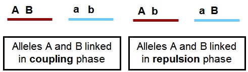
The picture shows two individuals carrying one chromosome from the mother (red) and one from the father (blue). The red and blue chromosomes are homologues of each other. They contain two linked loci, A and B, and each locus exists in two variants (alleles), indicated here as A and a, and B and b. Left: Alleles A and B are linked in coupling phase, and A and b in repulsion phase. Right: Alleles A and b are linked in coupling phase, and A and B in repulsion phase. The two loci are linked; the alleles are in coupling or repulsion phase.
Suppose that alleles A and B are favorable. In that case, the ideal genotype AABB can be obtained easily in the case of linkage of A and B in coupling phase (left): if the two loci are (closely) linked, selection for A will almost always also bring allele B to the same progeny (it requires only non-recombinant gametes). If the alleles are linked in repulsion, however, (right picture), it will be hard to obtain AABB, since they occur on two different homologous, so it requires a recombination event, in both gametes, between A and b to bring A and B together.
Show/hide comprehension question...
Show/hide comprehension question...
When genes are located on different (non-homologous) chromosomes, they inherit independently (see figure below). The process involved is called independent assortment of chromosomes. Whether a gamete receives homologue 1 or 2 of chromosome 1 has no relation with whether this gamete receives homologue 1 or 2 of chromosome 2. Genes on different chromosomes are always unlinked and their inheritance is independent.
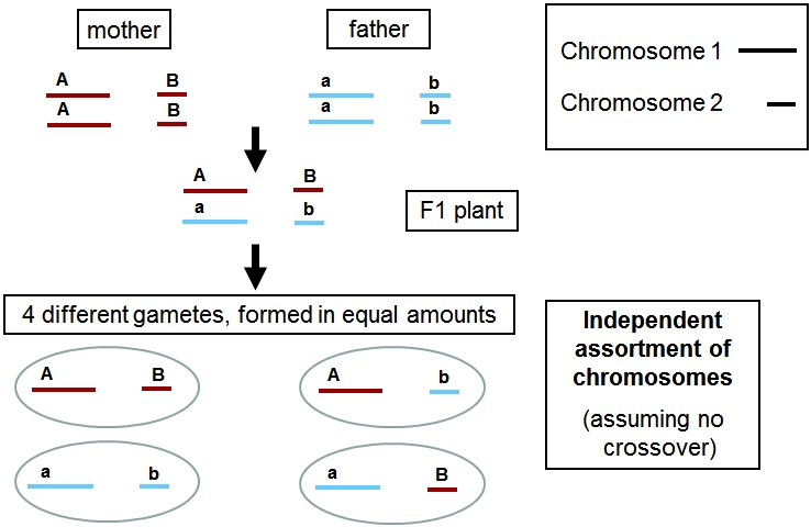
Independent assortment of chromosomes during meiosis results in random distribution of chromosomes per homologous pair. For example, a gene located on Chromosome 1 is not linked with a gene on Chromosome 2, and hence they are distributed independently from each other during meiosis. The chance for A and B ending up in the same gamete is as large as the chance for A ending up with b.
During a cross-over, homologous parts are exchanged, resulting in intrachromosomal recombination (= recombination within the chromosome between the homologues; see figure below).
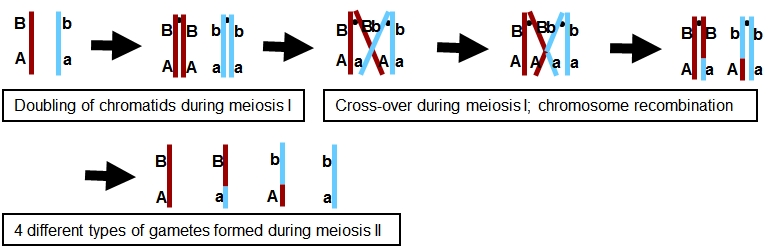
The meiosis depicted above will result in gametes AB, aB, Ab and ab. Of these, the aB and Ab gametes are novel (non-parental) combinations, hence the term 'recombination'.
Note that recombination only results in new allele combinations when homologues carry different alleles on both loci: both should be heterozygous (double heterozygous). If between loci A and B there are other sequence differences between the two parents, these will also form new combinations.
When genes or markers are located together (on the same chromosome), they are called 'linked'. The shorter the distance between them, the lower the chance for a cross-over taking place between them. Alleles of closely linked loci tend to inherit together, because the probability of a crossover event in between the two loci is rather small.
A linkage group is a statistically defined group of genes/markers that are significantly associated. This association is usually ascribed to physical linkage of their loci on the chromosome. In theory, a linkage group comprises all loci on an entire chromosome. The linear linkage of the loci causes the genes and markers to be linked to each other, and to inherit in association. However, in practice, linkage is not always statistically shown, e.g. because of large gaps due to insufficient markers or non-polymorphic chromosome regions.
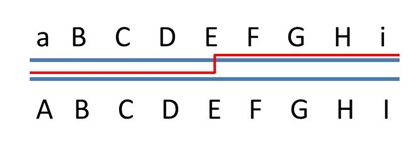
Genes (or a gene and a marker) that are located on the same chromosome, but far away from each other (like A and J in the picture below), behave as if they were unlinked. This is because, during meiosis, in the paired homologous chromosomes
there is such a high probability for one or more recombinations to occur, that in case of A-a/J-j polymorphism, A will roughly occur equally frequent with the linked J (gamete AJ) as with the alternative j (gamete Aj).
|
|
|
The loci on which genes or markers A to J are located are all linked. They form therefore one linkage group. The distance between locus A and J may be so large, that the linkage between these two loci is not statistically significant. |
Summary
→ Genes/markers are linked if they are located closely together on the same chromosome
→ Gene/marker alleles can be linked in coupling phase (on the same homologue) and in repulsion phase (on different homologues)
→ Independent assortment of chromosomes is the mechanism for non-homologous chromosomes to recombine
→ Cross-over is the mechanism for homologous chromosomes to recombine
→ A linkage group is a statistically defined group of genes/markers that are significantly associated
→ New combinations of alleles of (linked and unlinked) genes can only arise if those genes were both present in a heterozygous state.
I want an alternative explanation | Move on to: Linkage, recombination and map distance
Many crop species have two sets of chromosomes (i.e. they are diploid): one set inherited from the mother (e.g. the red chromosomes 1 and 2) and one set inherited from the father (the blue chromosomes 1 and 2). These are depicted in the figure below. Chromosome 1 from the mother and Chromosome 1 from the father are called homologues: they carry the same types of genes, but they can carry different alleles for those genes. A might be for flower color, A giving red flowers, a white, and B may be for hairiness of leaves, b being glabrous. In this example, a situation with two homozygous parents is shown.
Each chromosome consists of two chromatids that are identical up to the beginning of the meiosis, in which the gametes are formed.
During formation of sexual haploid cells (gametes) the chromosomes of each homologous pair are randomly distributed over the gametes, in such a way that each gamete receives one copy of each chromosome (so one of the homologues). For example, one gamete can contain Chromosomes 1 and 2 from the father, another can receive one from the mother and the other from the father, etc. Therefore, genes located on different chromosomes are inherited independently from each other: they are unlinked. Unlinked loci will show a recombination frequency of about 50% consistent with random assortment
Not all plant species are diploid and even within a species different ploidy levels can occur. In tetraploid species, e.g. each chromosome is present in four copies (4n): two from the mother and two from the father. In a hexaploid (6n), three from the mother and three from the father.
Confused about ploidy levels?
Test yourself and match the ploidy level with the number of chromosomes in a normal cell.
Show/hide comprehension question...
During meiosis, genes and markers segregate via interchromosomal recombination (independent assortment of chromosomes) and intrachromosomal recombination (cross-over). Genes or markers that are on loci close to each other ('tightly linked') on the same chromosome will be transmitted together from parent to progeny more frequently than genes or markers that are located further apart on the same chromosome.
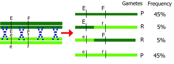
Effect of cross-over between homologous chromosomes.
Dark chromosomes originate from one parent; light chromosomes from the other parent. Only one chromosome pair is shown here. Note that during meiosis, each chromosome initially consists of two identical chromatids. P=parental, original, R=recombinant.
Gametes that are produced after meiosis either have the same combination as a parental chromosome (parental, P) or they have a different, non-parental combination (recombinant, R). The smaller the distance between two genes, the smaller the probability of recombination between the two genes.
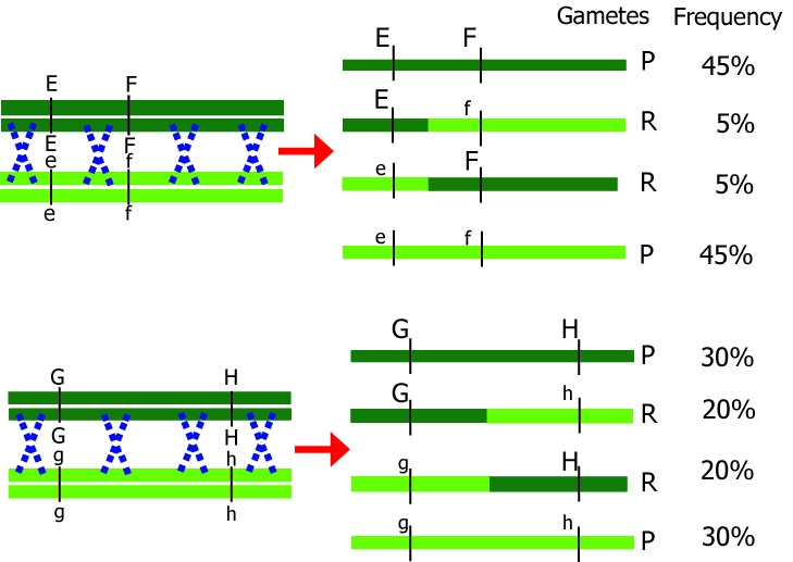
Different distances between genes result in different recombination percentages.
Note: The blue crosses in the figures do not indicate two recombinations at the same time, but rather that the chance for one recombination to occur is larger than when the loci of interest are closer to each other.
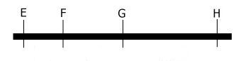
If loci are further apart, the chance of a crossover event occurring between them is larger. Therefore, recombination between loci G and H should occur more frequently than recombination between loci E and F. The other way around,
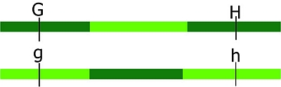
if we know the recombination frequencies, we convert these to genetic distances between the genes. Let us assume E, F, G, and H are loci in a population that segregates after crossing: from the number of recombinant individuals, it can be concluded that loci E and F are closer together than G and H.
More than one cross-over event can occur between loci. The probability of multiple recombinations increases with the distance between the loci. If two cross-over events take place between loci G and H in the same pair of chromatids, we would observe a non-recombinant genotype while in fact there was a double recombination event:
Keep in mind that: the closer to each other two loci are situated on a chromosome, the lower the recombination
frequency is. (And, the further away they are situated on a chromosome, the higher the recombination frequency between two loci). Markers located on different chromosomes are unlinked. Markers located far apart on the same chromosome are behaving as unlinked, because of high probabilities of one or more recombination events occurring. In a diploid, unlinked loci have an expected recombination frequency of 50%.
Often, the physical distance (in terms of DNA base pairs) between loci is not known. Recombination frequencies can be calculated in the offspring and be used to calculate the genetic distance between them.
The unit of genetic distance is the centi-Morgan (cM). A centi-Morgan map unit is defined as an expected cross-over frequency of 1 percent, or 0.01 per gamete formed. Generally, loci that have a recombination frequency of about 50% are considered 'unlinked'. However, they may belong to the same linkage group! The figure below shows a linkage map. This is a graphical representation of all the genetic positions of markers and genes relative to each other. Loci A and J at the far ends of the same chromosome behave as being not linked (recombination about 50%), since there will be a high frequency of one or more recombinations between them. They are, however linked via the loci B, C, ... and I.
![]()
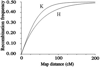
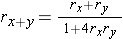
Mapping functions are used to convert recombination frequencies into cM map units. The relationship between map distance and recombination frequency is non-linear: when the distance increases, the recombination tends to 50%.
Recombination frequencies are non-additive due to the possibility of even numbers of recombination events which are not observed from the genotype frequencies. Map distances in cM units are additive. So, if a locus B is located between loci A and C, the distance in centiMorgan units between A and B and between B and C can be added up to give the distance between A and C. In contrast, the recombination frequency between A and C is smaller than the summed recombination frequencies of A-B and B-C due to the possibility of double recombination events: a recombination in both A-B and B-C does not lead to (observed) recombination between A and C, it would be observed as a non-recombinant rather than two consecutive recombination events. A recombination frequency estimate from an observed number of recombinant genotypes will therefore, especially for loci linked at larger distances, often be an underestimation of the true number of recombination events, crossovers.
Summary
→ A recombination frequency indicates genetic distances between a pair of genes, a pair of markers or a gene and a marker
→ The closer two loci are situated to each other on a chromosome, the smaller the recombination frequency, and vice versa
→ The farther apart two loci are on a chromosome, the closer to 50% the recombination frequency will be. Loci on different chromosomes have an expected recombination frequency of 50% as well, corresponding to independent segregation at the two loci.
→ Genetic distances are usually indicated in centiMorgan units rather than recombination frequency units since cM distances are additive and recombination frequencies are not
→ The relationship between recombination frequency and cM genetic distance is non-linear
I want an alternative explanation | Move on to: Why use linkage maps?
Diploid species have one set of chromosomes from the mother (let us call them m1 – m10 for a species with 10 chromosome pairs) and one from the father (f1 – f10): m1f1, m2f2, m3f3 …m10f10. Let's assume these parents have been crossed and we are considering the F1 of this cross. Sexual propagation (i.e. involving meiosis) is very important, because it favors efficient recombination of genes through two systems:
1. Cross-over between homologues in the F1 meiosis
This can occur between the chromatids of homologous chromosomes, so in this F1 between m1 and f1, and m2 and f2 etc. (m1 is one homologue of chromosome 1, f1 the other in the F1 of this cross)
This results in 'mixed' chromosomes, which contain pieces of m1 and pieces of f1, m2/f2 etc. Let us indicate them with m1' and f1' etc., depending on the chromosome (m1 or f1) from which they got their centromere.
2. Independent assortment of chromosomes in the F1 meiosis
After the first meiotic division, each cell contains one random copy of each chromosome, e.g. m1', m2', f3', m4', f5', f6', m7', f8', f9', m10', or any other combination.
The value of this recombination is that in the progeny the genetic information between chromosomes and within chromosomes is mixed to form novel combinations of genes. Most likely, there will be some progeny members with a combination of genes that is superior to the parent plants.
On the basis of recombination frequencies between loci, we may compare genetic distances between loci, and draw them on a linear map according to their estimated genetic distances. Such a drawing we call a linkage map. The most important use for linkage maps is to identify DNA regions that contain markers and genes that are associated with traits of interest. Linkage maps are also referred to as 'genetic maps'. Linkage maps result from statistical calculations of pairwise recombination frequencies between markers and/or genes and ordering and integrating them according to linkage groups, estimating their relative positions and distances. Linkage maps are useful in genetic research and in breeding, because:
Genes that contribute to quantitative traits are often found on different chromosomes. Knowing the number of genes that are associated with variation in the phenotypic trait tells us about the genetic architecture of a trat. It may tell us, for example, that plant length is controlled by many genes with small effects, or by a few genes with relatively large effects. The details of such quantitative trait locus analysis (QTL analysis) will be treated later.
Once the association between a gene and a marker is shown, markers can be used in breeding programs to select for desirable traits. We will see how this works in the following pages.
Alternatively, once a region of DNA is identified as contributing to a phenotype, the entire region can be sequenced. The DNA sequence of any gene in this region can then be compared to a database of DNA for genes whose function is already known, possibly also from genomic data of other plant species (e.g. the plant model species Arabidopsis thaliana)
The linkage map will show the distribution of markers over linkage groups, ideally corresponding to different physical chromosomes, and approximate positions of markers relative to one another on these linkage groups, and possibly also of markers relative to a linked gene in a genome region. The same linkage map or linkage maps developed on a mapping population developed from different parents, may contain additional markers that are also in that same region. Such additional markers may be used to screen material that segregates for the gene of interest to find markers that are even more closely linked to the gene. The closest linked markers may be used in marker-assisted selection for the trait conferred by the gene.
Summary
→ Linkage maps result from combining all the statistical calculations on recombination frequencies between all marker pairs and converting these into genetic map distances expressed in centiMorgan units
→ Linkage maps indicate which markers are linked and show their relative positions and genetic distances
→ Linkage maps are very useful in genetic research
→ Linkage maps are very useful in breeding for selecting markers that are linked to important genes that confer or contribute to traits of interest. In some cases, such markers may also be used to select in segregating populations for which no linkage map has been constructed.
→ A linkage map can be used to show the approximate position of a qualitative trait gene relative to linked markers, and may suggest which markers in the gene region may be developed as selection markers if these are even more closely linked to the gene of interest.
Show/hide comprehension question...
I want an alternative explanation | Move on to: How to make a linkage map
A linkage map is a graphical representation of all the genetic positions of markers (and sometimes genes of monogenic traits) relative to each other.
First, a set of genetic markers must be developed. Then, a population is scored for polymorphic markers. Statistics will show which markers are linked on the same linkage group. In addition, the recombination frequencies between markers can be used to estimate their order and genetic distances. This way, per linkage group a linear map can be drawn showing the estimated order and approximate distances between marker loci.
Markers are easily made visible. Scoring for traits is often laborious. Selection for favorable genes may be substituted by selection for a linked marker. This can also be done in other populations (e.g. breeding populations), if the marker also
segregates in those populations. So, ideally, creating the map is a one-time effort after which the map can be used many times.
Linkage maps are constructed on the basis of analysis of many segregating markers in a large segregating population. The three main steps that lead to the development of a linkage map are as follows:
(1) Development of a mapping population
(2) Genotyping: identification of polymorphism of markers in parents and progeny and running the markers
(3) Linkage analysis of markers: determining the degrees of associated segregation between markers (and possibly between markers and a gene for a trait) and construction of a genetic linkage map
After the linkage map has been constructed, these steps can be followed by:
(4) Phenotyping: scoring phenotypic traits in a mapping population, needed to later find associations of markers to phenotypic traits in a QTL analysis or in a linkage analysis of a qualitative monogenic trait (see 3)
(5) QTL analysis: establishing which regions in the genome are associated with a quantitative phenotypic trait
Ideally, once the linkage map is available, this map gives valuable knowledge of markers and their position on the genome. Such information can be used to locate genes in the original mapping population. But other segregating plant material (e.g. progeny of a cross of different parents) may also be genotyped with these markers, to find associations with some traits of interest. If such an association is found, we may conclude from the known position of the marker on the linkage map, that in that other material the gene for the associated trait should be in the same chromosome region. However, many markers used to create the map, might not be polymorphic in the other population. Also, the trait of interest might be influenced by different genes in different populations, because some genes might be polymorphic in the mapping population and not polymorphic in the new population and vice versa. This will be explained in further detail later on.
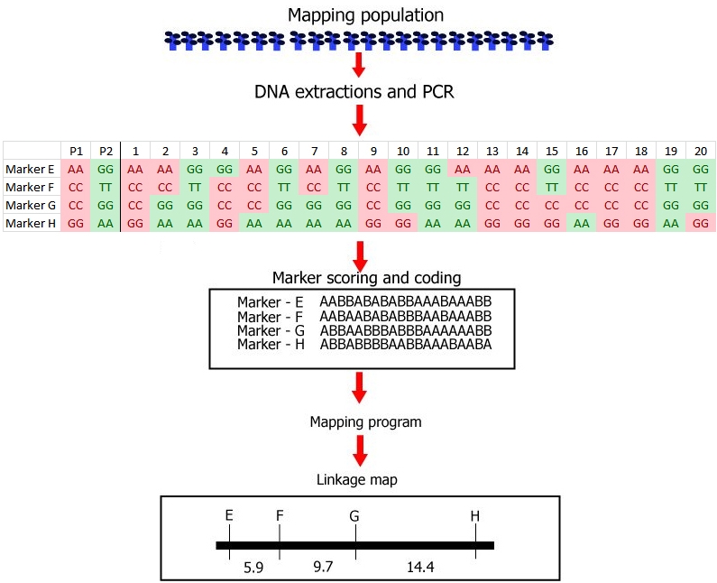
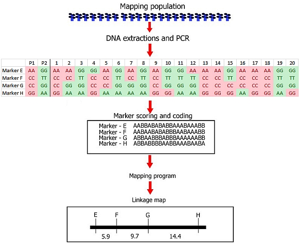
Steps involved in the construction of a linkage map with DNA markers.
(1) Development of a mapping population: this example is based on a small recombinant inbred population (RIL) from a cross, consisting of only 20 RIL individuals. Note that this low number of individuals is not realistic. In the real world, the mapping population should be large (a large number of RILs in this case): in small populations linkage between markers and markers and associations between markers and a trait cannot be established with any reliability.
(2) Genotyping: DNA extraction and PCR, followed by:
Identification of polymorphisms and running the markers: the first parent (P1) is scored as an 'A' whereas the second parent (P2) is scored as a 'B' for each marker; each individual is scored likewise. In this case 'A' refers to the homozygous diploid genotype of an individual equal to the parent P1 genotype (e.g. MM), and 'B' to the homozygous diploid genotype of an individual equal to that of parent P2 (e.g. mm).
(3) Linkage analysis: estimation of recombination frequencies of all marker pairs and sometimes of genes for qualitative traits. Determine which markers and genes are linked, and constuct a genetic linkage map by assignin
g markers to linkage groups, establishing marker order, and genetic distances in cM units per linkage group.
After the linkage map has been constructed, these steps are followed by:
(4) Phenotyping: Scoring of phenotypic traits in a mapping population,needed to later find associations of markers to phenotypic traits in a QTL analysis or in a linkage analysis of a qualitative monogenic trait (see 3)
(5) QTL analysis: establishing which regions in the genome are associated with a quantitative phenotypic trait
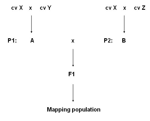
To make a linkage map, first we need a segregating plant population. This is a population resulting from sexual reproduction. The production involves:
Summary
→ To create a linkage map, a segregating plant population must be "genotyped" for the marker alleles occurring in each member of the population
→ The parents of a mapping population are usually chosen to contrast in traits of interest, but the same population may be also used for other traits
→ For a mapping population in an autogamous crop the F1 of a cross should be heterozygous for many markers and for the traits of interest. For a mapping population of an allogamous crop, at least one parent must be heterozygous for markers and the traits of interest.
I want an alternative explanation | Move on to: Development of a mapping population in autogamous species
A mapping population needs to have diversity in traits (must be segregating). In autogamous crops, this is often achieved by crossing rather contrasting parents. The two parents of a mapping population:
In most crops, the number of polymorphic markers is sufficient to develop linkage maps.
In autogamous species, mapping populations usually originate from the F1 of a cross of inbred lines: each parent is homozygous and the F1 is heterozygous at the loci at which the parents have different alleles. The segregation among these parental alleles when the F1 pollen and F1 egg cells are formed is studied in a linkage analysis of genotypes in F1 derived populations, such as the ones shown below.
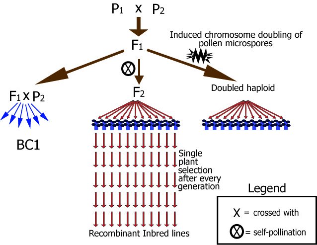
Diagram of main types of mapping populations for autogamous species.
In this figure, for example, Parent 1 (P1) could be AABBCCDDEEFFGGhh and Parent 2 aabbccddeeffGGhh, each letter representing an allele of a gene or marker. These examples are chosen for simplicity, but any other homozygous combination like AAbbccDDEEffGGhh and aaBBCCddeeFFGGhh could also be possible, as long as there is sufficient difference between the parents: in this example, polymorphism is present for six markers or genes (and absent for two). The resulting F1 population consists entirely of AaBbCcDdEeFfGGhh plants. Note that in this example the F1 is homozygous for the G and H locus only. After that, there are different ways to create segregating populations:
|
Population type |
Codominant markers |
Dominant markers |
|---|---|---|
|
F2 |
1 : 2 : 1 (AA:Aa:aa) |
3 : 1 (B_:bb) |
For a codominant gene or marker (for which AA plants can be distinguished from Aa plants), Aa x Aa results in an expected segregation of 1:2:1 (AA:Aa:aa).
For a dominant gene or marker Bb x Bb results, by expectation, in 3:1 (B_:bb).
F2 progenies in autogamous crops have been often used for construction of genetic maps and for studying monogenic traits. They are less useful for QTL analysis, genetic studies of quantitative traits or traits requiring much plant material of a , for two reasons:
F2 can be suitable for such analyses if the plant species is a perennial or if it can be vegetatively propagated to create clones. Sometimes the F2 is used for map construction while phenotyping is done in the F3 lines derived from genotypes F2 plants.
Selfing of individual F2 plants for a number of generations allows the development of recombinant inbred lines (RILs), which consist of a series of homozygous lines, which can be reproduced identically. It should be mentioned that some heterozygosity may still be present in RIL lines, especially if they are not from many generations of selfing.
How to develop RILs?
In a population of about 200 F2 plants, we harvest one seed per plant. Or better, two seeds to keep one as back-up, in case the first fails to germinate or to develop a next generation of seeds. We repeat this each generation. Harvesting and propagating in each generation one seed and one plant per original F2 plant is called single seed descent (see module on Principles of Plant Breeding - Selection methods; abbreviated to SSD).
At about the F7 or F8 we may presume that each of the plants is homozygous for the great majority of loci for which the parents originally carried different alleles. In the F7, a plant is probably heterozygous for about 1/64 of all loci that segregated in the F2.
The resulting set of about 200 homozygous plants, each derived from a different F2 plant of the same cross can be propagated by selfing. So, they can be phenotyped at population level in replications, and maintained infinitely: they are "immortal".
(Of course, an 'immortal' line can die, as a result of disasters or extreme weather conditions killing all plants, and when also the stored seed is lost). "Immortal" here refers to the genotype of the individuals, that can be reproduced identically for many generations, not to the individuals themselves, and as a contrast to the F2, for example, which can not be reproduced identically by fertilized seeds in the following generation.
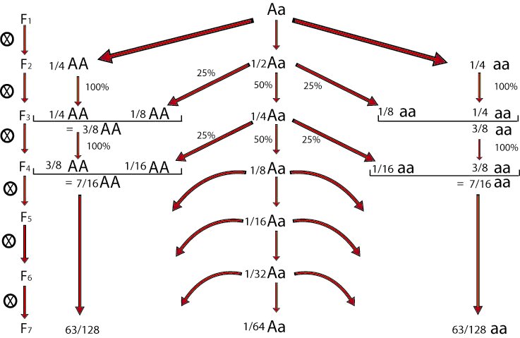
After six to eight generations, there will be homozygosity at most loci:
Plants homozygous at a locus produce 100% homozygous offspring for that locus and plants heterozygous at a locus produce 50% homozygous and 50% heterozygous offspring for that locus. The proportion of heterozygotes is halved in each generation. In every generation there is meiosis and there are possibilities of recombination as long as a chromosome segment still has heterozygous regions.
The resulting RILs each contain a unique combination of chromosomal segments from the original parents.
|
Population type |
Codominant markers |
Dominant markers |
|---|---|---|
|
F2 |
1 : 2 : 1 (AA:Aa:aa) |
3 : 1 (B_:bb) |
|
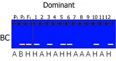
Backcross BC1 |
1 : 1 (Cc:cc) |
1 : 1 (Dd:dd) |
For a codominant gene or marker Cc x cc results in a segregation of 1:1 (Cc:cc).
For a dominant gene Dd x dd this is exactly the same: 1: 1 (Dd:dd) (Table).
Note that if the F1 is backcrossed to recurrent Parent 1 (Cc x CC), the result is a segregation of 1:1 (CC:Cc) for a co-dominant marker. For dominant markers we get 100% D_. So only markers can be used to genotype the mapping population that are co-dominant or for which the recurrent parent is homozygous recessive.
Note that the backcross population is compared to the F2 population equally mortal and equally confined to individual, genotypically unique plants.
|
Population type |
Codominant markers |
Dominant markers |
|---|---|---|
|
F2 |
1 : 2 : 1 (AA:Aa:aa) |
3 : 1 (B_:bb) |
|
Backcross |
1 : 1 (Cc:cc) |
1 : 1 (Dd:dd) |
|
Recombinant inbred lines or doubled haploids |
1 : 1 (EE:ee) |
1 : 1 (FF:ff) |
In a number of crop species, haploid plantlets are induced to develop from microspore cells or from certain prickle-pollinated egg cells. For several crops specific methods have been developed to induce such haploids out of male or female gametes. Those haploid plants may spontaneously or induced by chemicals double their chromosome numbers to result in a doubled haploid (DH). A segregating DH population can be obtained by inducing doubled haploids from an F1 plant (from a cross between homozygous parents). The Ee plants produce E and e gametes in roughly equal ratios. Doubling of chromosomes of the haploids results in 1:1 (EE:ee) plants, which segregate equally for the genes and markers for which the parents differed in allele. Note that this results in plants that are homozygous on all loci. Different plants however will be different homozygotes. For example, one plant might have the AAbbCCDDeeFFGGhh genotype whereas another might have the aabbCCddEEffGGhh genotype. The resulting set of about 200 DH plants are homozygous, each derived from a different gamete of the same heterozygous plant, and can be propagated identically by selfing. So, as with RILs they can be phenotyped at population level in replications, and maintained infinitely: they are "immortal".
Note that if F1 plants might be genetically different (because of non-homozygousity at some loci in a parent plant), the DH population should preferably be derived from a single F1 plant.
The DH plant is the result of only a single meiosis so that there is only one opportunity for recombination to occur: the meiosis in the F1 plant that produces the gametes that are used to induce the haploids. The next stage is already the DH population, in which selfing cannot increase the number of recombinations since the plants are already fully homozygous. There is a very different situation during the development of a RIL population. In a RIL population, there are not only the recombinations that occurred in the F1, but also in the heterozygous chromosome fragments in the F2 and in those in the F3 etc. The later the generation, the less chance for such heterozygous fragments in which additional recombinations may occur. Also, the plants at the start of the SSD procedure to create the RILs were the result of two gametes, and of the DH plant of only one gamete. The additional recombination opportunities together with the higher diversity at the start results in more recombinations than in the DH population. This results in a larger resolution of the map in RIL populations than in DH populations.
|
Population type |
Codominant markers |
Dominant markers |
|---|---|---|
|
F2 |
1 : 2 : 1 (AA:Aa:aa) |
3 : 1 (B_:bb) |
|
Backcross |
1 : 1 (Cc:cc) |
1 : 1 (Dd:dd) |
|
Recombinant inbred lines or doubled haploids |
1 : 1 (EE:ee) |
1 : 1 (FF:ff) |
→ Summary of advantages and disadvantages of mapping populations developed for autogamous species is listed in this table:
|
Mapping population |
Origin |
Advantages |
Disadvantages |
|---|---|---|---|
|
F2 |
F1 selfed |
|
|
|
Backcross (BC1) |
F1 x parent |
|
|
|
Recombinant inbred lines (RILs) |
Selfing of F2 for a number of generations |
|
|
|
Doubled haploid (DH) |
Induced chromosome doubling in gametes |
|
|
Show/hide comprehension question...
In allogamous species, the situation is often more complicated than in self-pollinated species. Forced and repeated self-fertilisation often leads to inbreeding depression, i.e. inferior and stunted plants. As a consequence, RIL populations cannot be developed. Due to the poor tolerance of homozygosity, also DH populations are often not an option either. However, notable exceptions exist, for example maize, which is naturally cross-fertilizing but can be selfed without problems. Other outcrossing organisms, like animals (e.g. mice or Drosophila) can be inbred by brother-sister matings.
In allogamous species, mapping populations are created developed by crossing two heterozygous parents, or by selfing one single (heterozygous) plant. Since in cross-fertilizing species often F1 hybrid cultivars are developed, or highly heterozygous plants are clonally propagated (apple, potato), one selfing of such plant will result in segregation of all the marker and gene loci that were heterozygous in the parental plant.
Due to the high level of heterozygosity, there is a much greater need for co-dominant markers in allogamous crops. This situation is very different from the autogamous crops treated on the previous section, since in autogamous crops,
RIL and DH populations can be used and co-dominance of markers is not so important (only homozygotes need to be distinguished).
Some crop species are polyploid, i.e. they contain more than two copies per chromosome. Tetraploids have four homologues of every chromosome, hexaplois have six, octoploids eight. This situation presents a problem during genotyping and genetic analysis, since, per locus, different types of heterozygotes are possible, which are hard and sometimes impossible to distinguish (AAAa:AAaa:Aaaa). Recently, software has been developed for so-called dosage scoring of SNP markers, so that, e.g. for a tetraploid crop, all five possible dosage classes (nulliplex, simplex, duplex, triplex, quadruplex, for aaaa, Aaaa, AAaa, AAAa and AAAA, respectively) may be distinguished. Often, not all five classes are present and fewer classes need to be distinguished. Still, it may happen that for individual SNPs, the classification is very difficult.
Moreover, during the mapping of a polyploid species, there can be uncertainty about whether a certain allele originated from the father or from the mother (if both parents are heterozygous). Also, during meiosis, preferential pairing may have occurred: homologues from one parent might pair together more frequently than with homologues from the other parent. At meiosis, complex chromosome pairing patterns may occur, involving more than two chromosomes. These are called trivalents, quadrivalents, etc., according to the number of chromosomes participating in the pairing complex. Such multivalents may recombine chromosome fragments between more than two chromosomes, and are therefore more complex to study than recombination in diploid parents, where only bivalents occur.
A solution to overcome these problems is the mapping of only simplex X nulliplex markers that are in coupling phase with each other, these are all from the same homologue (simplex = recessive at all alleles of a gene except one; nulliplex = recessive in all alleles of a gene; e.g. in tetraploids: Aaaa X aaaa). This situation is similar (with respect to recombination frequency estimation, ordering and distance determination) to a backcross in diploids (Aa x aa), though not identical.
It may also be possible to map simplex X simplex (=Aaaa x Aaaa) or duplex X nulliplex markers (AAaa x aaaa or aaaa x AAaa). More complex situations are not treated here.
Another option is to construct a linkage map using diploid relatives of the polyploid crop species. However, these do not always exist, but may be developed in the same way as haploids are induced in diploid species and even if they do,
it is still far from straightforward to translate results back to the polyploid level at which research and/or breeding is usually done.
Summary
→ In autogamous plant species, a linkage map can be created, based on a population (F2, backcross, RIL or doubled haploids) derived from homozygous inbred parents
→ In allogamous plant species, a linkage map can be created, based on an F1 population derived from a cross between heterozygous parents or on a progeny from selfing of one single heterozygous plant.
→ Mapping of polyploid plant species is often performed on simplex X nulliplex markers
→ Sometimes, mapping of polyploid plant species can be aided using diploid relatives
|
|
|
Steps involved in the construction of a linkage map with DNA markers. |
As we have seen before, the three main steps of linkage map construction are:
(1) Development of a mapping population
(2) Genotyping: identification of polymorphism of markers in parents and progeny and running the markers.
(3) Linkage analysis of markers: determining the degrees of associated segregation between markers and construction of the linkage map
After the linkage map has been constructed, these steps are followed by:
(4) Phenotyping: collect trait values for QTL analysis or mapping of a qualitative trait
(5) QTL analysis
The second step in the construction of a linkage map is to identify DNA markers that reveal differences between alleles (i.e. polymorphic markers), and run them on the members of the mapping population. This running of markers on a mapping population is called genotyping. It is critical that sufficient polymorphism already exists. For mapping populations derived from homozygous parents, these parents are usually chosen on the basis of a clear contrast in the trait of interest and on a high expected level of polymorphism over the genome. Usually any pair of cultivars shows polymorphism. However, in some crops, e.g. tomato, genotypic uniformity is very high, and lack of polymorphism may be a problem. Generally, the less related (for example if collected on different continents) the higher the genetic variability and hence the degree of polymorphism. When there is no polymorphism, no linkage map can be made. If two parents share one of their ancestors, some parts of their genome may be not polymorphic.
|
|
|
If cv A and cv B share cv X as ancestor, some parts of genome of A will be derived from X, and in cv B also parts of the genome are derived from cv X. For some of the chromosome fragments those X-derived fragments are the same in A as in B, and therefore carry the same marker and gene alleles, and hence are not polymorphic. |
Once polymorphic markers have been identified, they must be screened across the entire mapping population, including the parents. This is known as marker genotyping of the population.
Before markers can be scored, DNA must be extracted from each individual of the mapping population and from the parents. There are several DNA isolation techniques. Since usually large numbers of plants should be sampled, a quick method is desirable. Such quick methods are available, but they tend to give a bit less reliable patterns when processed to reveal markers. More laborious methods may give a more stable and reliable marker pattern, and the DNA may be stored longer. For markers that are based on Southern Blotting (RFLP) much larger amounts of DNA need to be sampled than for markers that depend on PCR amplification. That is one of several reasons why RFLP markers became obsolete.
Errors
Recording should be done very carefully: errors are a very common and disturbing factor in map construction. Sources of errors include unclear signals on the gel or blot, and simple typing errors in the spreadsheet. In case of a doubtful signal on the gel, it is better to enter a missing value symbol in the data sheet. The reason for this is that genotyping errors will often count as extra recombinants in the data analysis, and often even as 'double recombinants' (both to the left side and to the right side of an incorrectly scored marker, a false 'recombination' is observed). Errors in genotyping increase the length of genetic maps, cause incorrect ordering and distance estimation among markers and reduce the power of gene detection and QTL analysis and decrease the accuracy of the results, for example of the estimated effects of genes or QTLs on a phenotypic trait
Examples
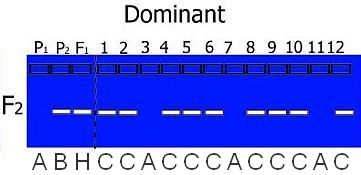
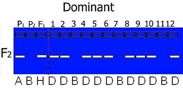
Examples of DNA markers screened across different populations are shown in the figure below.
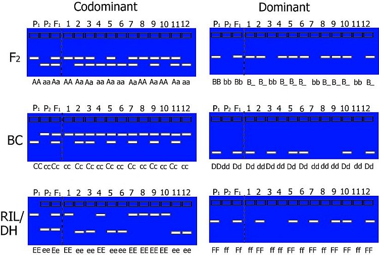
Hypothetical gel photos representing segregating codominant markers (left) and dominant markers (right) for typical mapping populations. Codominant markers reveal the complete genotype for a marker. Note that dominant markers cannot discriminate between heterozygotes and one homozygote genotype in F2 populations.
The expected segregation ratios for codominant and dominant markers are presented in the table. Significant deviations from expected ratios can be analysed using chi-square tests. Generally, markers will segregate in a Mendelian fashion.
Sometimes, distorted segregation ratios may be encountered so that we cannot always assume nice 1:1, 1:2:1 or 3:1 segregations in a progeny. Be aware that deviations from these expected segregation ratios might be caused by scoring difficulties or quality issues (bad quality DNA, for example) but also by biological phenomena (gametophytic or zygotic selection, self-incompatibility, or deleterious loci). However, scoring difficulties and quality issues would usually be observed at individual loci, while neighbouring markers are unaffected, whereas biological phenomena would usually affect a number of markers in the same genomic region.
|
Population type |
Codominant markers |
Dominant markers |
|---|---|---|
|
F2 |
1 : 2 : 1 (AA:Aa:aa) |
3 : 1 (B_:bb) |
|
Backcross |
1 : 1 (Cc:cc) |
1 : 1 (Dd:dd) |
|
Recombinant inbred or doubled haploid |
1 : 1 (EE:ee) |
1 : 1 (FF:ff) |
Note: larger numbers of markers are usually indicated with M1, M2, M3 etc., also to avoid confusion with the coding explained in the next paragraph.
In the examples above we have given the allele names of the markers, e.g. AA, Aa and aa, and BB, Bb, B_ and bb, but in the case of progenies from homozygous parents, for large numbers of markers a special type of coding is used:
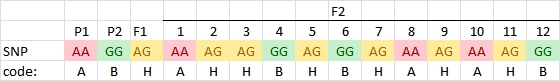
However, in the case of a dominant marker in an F2 population, we cannot tell if an individual is heterozygous or homozygous for the dominant marker allele. We only know that it is not homozygous for the null allele. In those cases we need more codes:
Coding is dependent on the type of mapping population used. For example, in a RIL or DH population only homozygotes are present (so codes H, C or D do not appear in the offspring) and in a BC population, we know that heterozygotes are present and only one type of homozygote: the one from the parent used for backcrossing:
In practice, you also may have missing data or bands that are unclear. These receive a special code U.
Coding in F1 progenies of crosses of heterozygous parents of an allogamous crop is different, and even different for different markers, since different segregation types may be present at the same time: for some markers P1 will be heterozygous and P2 homozygous; for other markers P1 may be homozygous and P2 heterozygous, while for again other markers P1 and P2 may both be heterozygous for the same alleles or for different alleles. In polyploid crosses the coding is again different because dosage differences need to be taken into account as well as heterozygosity/homozygosity, but this will not be treated here.
Even though it is, by far, preferred that the parents of a mapping population are also genotyped for all the markers, map construction is still possible if one or both parents are missing. The coding then has to be adapted to reflect this uncertainty.
Summary
→ To identify and score polymorphic DNA markers, DNA must be extracted from each individual plant in the mapping population and the parents
→ Segregation of markers generally follows a Mendelian fashion, but distorted segregation is not uncommon
→ Codes used for genotyping as used in mapping programs such as JoinMap and MapQTL are listed in the table above
I want extra information | Move on to: Step 3. Linkage analysis of markers
Watch this animation on gene mapping, using RFLP markers. RFLPs are not used anymore, but the principle of gene mapping remains.
|
|
|
Steps involved in the construction of a linkage map with DNA markers. |
As we have seen before, the three main steps of linkage map construction are:
(1) Development of a mapping population
(2) Genotyping: identification of polymorphism of markers in parents and progeny and running the markers
(3) Linkage analysis of markers
After the linkage map has been constructed, these steps are followed by:
(4) Phenotyping: to go from the linkage map to QTL analysis
(5) QTL analysis
After having recorded the genotype of each individual of the mapping population for each segregating marker as A or B, we can perform a linkage analysis: i.e. we determine whether some markers tend to segregate in association with each other (or not at all). Computer software has been developed to perform such an analysis.
We now roughly illustrate the simplified process of linkage analysis, for four hypothetical markers, located on the same chromosome. For simplicity, we show only the data for the first 20 individuals out of a population of 200 individuals.
It is obvious that the markers show an associated segregation. An individual with the genotype of parent A for marker E has a high probability to carry also the alleles of parent A for the other markers. This association indicates linkage. For the markers E-H in the picture above, we can manually observe per marker pair the number of individuals that carry for one marker the allele of one parent and for the other the allele of the other parent (due to recombination, non-parental genotypes):
E and F: 2 individuals differ
E and G: 5
E and H: 9
So E and H will probably be further apart on the chromosome than E and F (more differences, more recombinants between these markers. However, from this information alone we do not know what the order of the markers and their distances on the chromosome will be. All these orders are possible (differences indicated with dots):
E..F...G....H
F..E.....G....H
G...F..E.........H
More information is obtained if we include the data of other markers:
F and G: 3 individuals differ
This results in possible orders:
E.F...G...H
G...F.E........H
G and H: 4 individuals differ and F and H: 7 individuals differ
These data together result in the most probable order:
E..F...G....H
Linkage map, as determined in our example.
Summary
→ Linkage of marker alleles can be analyzed by assessment of the amount of recombination.
I want extra questions on linkage analysis | Move on to: Linkage analysis in practice
For a few markers, linkage analysis can in some cases be performed manually, but for large numbers of markers, or situations with dominant markers or varying numbers of missing values, computer programs are needed. Commonly used software programs for construction of a linkage map include Mapmaker and JoinMap. These programs calculate/estimate all pairwise recombination frequencies between markers and determine the significance of linkage or of 'association'. The evidence of linkage is often quantified in a LOD score: the Logarithm Of Odds, which is the ten-based logarithm of the ratio of the likelihood of the observed genotype frequencies under linkage versus the likelihood in case the markers would be unlinked.
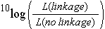
Usually, to construct linkage maps, the threshold value for the LOD value of two markers to be linked is set to a value between 3 and 4 (LOD threshold for linkage). This threshold can be defined by the user of the software or it can be indicated by the computer program, or the effect of different thresholds could be compared. A LOD threshold of 3 means that linkage between two markers, given the genotype frequencies, is 1000 times more likely than if markers were unlinked (3 is the 10log of 1000). A lower LOD threshold corresponds to detecting linkages under a relatively low significance level, whereas a higher LOD threshold would be more stringent: they tend to lead to decisions that markers that seem loosely associated are unlinked. However, the LOD threshold of 3 corresponds to a confidence level of about 95%. About 5% of the indicated linkages may be actually false positives: some of the (slightly) associated markers only are associated by chance and not by true linkage. This can be very undesirable since it might result in joining linkage groups that in reality correspond to different chromosomes. Also markers might be assigned to linkage groups based on not accurate enough information, for example if they show distorted segregation, had poor signals on the gel, or were entered with some trivial errors.
|
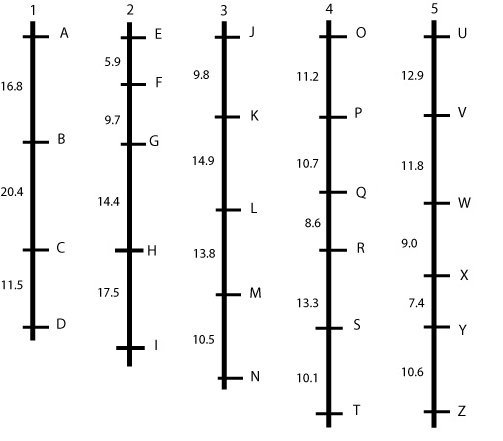
|
Hypothetical linkage map, consisting of five linkage groups (each probably representing a chromosome) and 26 markers. This picture represents an ideal situation, where markers are more or less evenly spaced. In a real situation, this is almost never the case, but we will observe gaps and clusters (see next example). The figures give the percentage of recombination between adjacent loci that is observed in this mapping population.
|
An ideal but unrealistic linkage map is shown in the figure above: linked markers are about evenly spaced and grouped together into 'linkage groups,' which, in an ideal situation, represent entire chromosomes or parts of chromosomes. Mostly, we prefer a linkage map with "spaces" of at most 5 cM between loci, so this map is not yet sufficiently "saturated".
In case we find large gaps, we should try to find more polymorphic markers between the parents and run those markers, hoping that some of them will map in the middle of some of the largest gaps.
Linkage maps may (at some chromosome regions) be more dense than necessary for mapping genes. This may be the case where thousands of markers were mapped, or in places where marker loci clustered, i.e. many markers map to almost the same locus (see for example in the middle of chromosome 3 in the figure below). We may, for further application of the map, delete most markers from the data set, and only retain the most reliably scored ones (with fewest missing data), with intervals of about 5 cM. Such a map is called "skeletal linkage map". This helps to reduce computational time for some calculations involved in map construction.
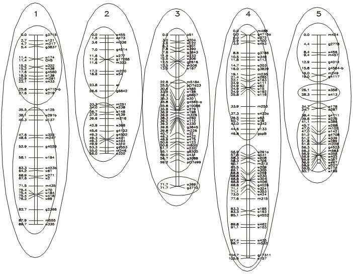
Assignment of markers to linkage groups at LOD = 12.0 (inner circles) and LOD = 5.9 (outer circles). (Maps calculated according to the (correct) assignment of 5 linkage groups, presumably located on 5 chromosomes).
Data source: Lister & Dean, Arabidopsis thaliana. Picture source: P. Stam, Study guide for the Wageningen MSc. course 'Modern statistics for the life sciences'.
The figure above shows a real-life situation of the assignment of markers to linkage groups, including clusters and gaps. Notice that a stringent (high) LOD threshold leads to more linkage groups than the haploid chromosome number.
When constructing a linkage map from scratch (with a set of markers that have not previously been assigned to linkage groups or chromosomes) it is recommended to stay 'at the safe side' by using a relatively high LOD threshold. This will prevent that groups of markers that in reality are on different chromosomes are incorrectly assigned to the same linkage group. Anchor markers known from other data sets may help to correctly group different linkage groups.
In the end, the number of linkage groups should be the same as the number of chromosome pairs in the organism's diploid genome (for autogamous crops; for cross pollinated crops often maps per parent are made, so there it could be twice the number of haploid chromosomes; for polyploids it could again be different, depending on the level of integration; e.g. for a tetraploid it could be either 1 linkage group per chromosome, 2, or 8). Assigning chromosome numbers to the linkage groups is done on the basis of (historical) knowledge on the location of certain morphological markers, resistance genes and standard markers mapped in other studies on the same organisms, and that are included in the present study as well, or, for sequenced crops, based on sequence information of these markers on the chromosomes.
Summary
→ A LOD score quantifies the strength of evidence of linkage (or sometimes of dependence) between markers based on genotype frequencies observed in the mapping population
→ The LOD threshold is a threshold above which genes/markers are considered linked
Show/hide comprehension question...
In this case study, a RIL population of 103 lines is created using the homozygous barley lines L94 and Vada as parents. The parents and the mapping population were phenotyped for their response to a certain disease resistance (R) or susceptibility (S) and genotyped for SNP markers. The picture shows data of the parents and, for simplicity, just 24 of the RILs and only few of the hundreds of segregating SNP markers. The bottom row presents the phenotyping data: resistant (R) or susceptible (S). The picture indicates a clear linkage of the resistance to marker M3. Two recombinations between M3 and the resistance phenotype occur (progeny lines 14 and 21). This implies that the marker is some distance away from the resistance gene. Maybe an additional marker will show a perfect association, and should then be closer to the R-gene locus (assumping perfect classification of the resistance in R and S). As expected the M3 marker allele of Vada (green) is associated with the Vada allele of the resistance gene. If we know the position of M3 on the linkage map, we also know the approximate position of the R gene. If the resistance is due to one gene, and the allele (R versus S) can be scored reliably, we may determine the position of the R locus as precisely as the position of each marker. We just add the R and S data in terms of A, B (in other populations also C and D), as done with markers, and the software can calculate its position on the linkage map.
This procedure is only possible for qualitative traits that can be classified into (in this case two) discrete classes according to their resistance genotypes (phenotype = genotype) and that are monogenic. If the resistance was classified into three or five categories, or if the resistance would be based on more than a single locus, no marker would have a perfect association with the resistance and the resistance could not be mapped as if it was a marker. Mapping procedures assume that each of the scored markers has a single position in the genome).
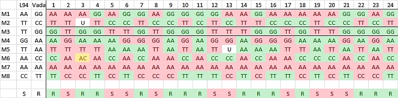
Observed linkage between resistance and SNP markers. Marker M3 is most probably located close to the resistance gene.
Extra discussion on this table:
Show/hide comprehension question...
Maps can be used to find markers linked to or in the region of genes for traits of interest. The marker loci are usually not evenly distributed over the chromosome, but they appear more clustered in some regions and absent in others (gaps in maps). Markers in clusters may be removed from the data set, to obtain a skeletal linkage map for application in mapping. Markers that have (nearly) the same segregation pattern, because of (near-) identical position are redundant: they do not add much power or precision to the outcome of the mapping study, but may increase computional time for analyses. In addition, in the case of even a low percentage of errors in genotyping, a large number of markers may drastically overestimate the map length of linkage groups because such errors cause an overestimation of the number of recombinations.
The recombination frequency is not equal along chromosomes: there are recombination 'hot spots' and 'cold spots'. Higher levels of recombination correspond to larger genetic map distances (more cM). Hot spots will therefore result in relatively large distances between adjacent marker loci. Cold spots will be 'condensed' on the linkage map: marker locus intervals are small, and markers tend to cluster. In many organisms, centromeric regions are cold spots, and often stand out in linkage maps as clusters of marker loci. In such cold spots there is hardly any relationship anymore between physical distance in base pairs (may be quite large) and genetic distance (0 or close to 0). In general, because the recombination frequency varies along chromosomes, the distances on a linkage map do not correspond to physical distances between markers measured in nucleotide base pairs.
Map distances are expressed in centiMorgan units (cM). When map distances are small (<10 cM), the map distance in cM is almost equal to the recombination frequency in percentage (per meiosis). However, when map distances are greater than approximately 10 cM, the map distance deviates more and more from the recombination frequency. This is because of the higher probability of multiple recombinations (see paragraph on 'Linkage, recombination and map distance') and interference caused by other cross-over events. The recombination frequency in a diploid cannot be higher than 50% (apart from some sampling variation), while the length of a linkage group corresponding to a single chromosome might be more than 100 cM.
Many of the markers observed in the population under study might be absent (or better: not polymorphic) in other populations. Therefore, they will not show up in linkage maps from other populations. Markers that are present in several maps can be used as reference for the location of other markers; these are called 'anchor markers' (will be treated in more detail later).
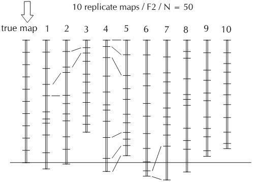
The accuracy of the map (marker order and distances) is directly related to the size of the mapping population. Mapping populations should consist of a minimum of 50 individuals (or lines) for constructing linkage maps. However, for application of mapping genes for traits of interest, especially mapping of genes with small effects (QTLs) a mapping population of about 200 genotypes is required. The larger the population the larger the power for detection of QTLs.
Interference means that crossover events in adjacent intervals interfere: the occurrence of an event in a given interval may reduce or enhance the chance for occurrence of an event in its neighborhood. Negative interference refers to the 'enhancement' of crossover events around a given one. Positive interference refers to the 'suppression' of crossover events in the neighborhood of a given one. In most organisms positive interference has been observed, to various degrees of intensity. Positive interference results in fewer double recombinants (over adjacent intervals) than would be expected on the basis of independence of recombination events.
Summary
→ The strength of evidence of linkage between markers is often expressed as a LOD score
→ Map distances are calculated from recombination frequencies and expressed in centiMorgan units
I want an alternative explanation | Move on to: Genetical map vs. physical map
Markers on non-homologous chromosomes inherit independently, because of independent assortment of chromosomes. Markers on homologous chromosomes inherit in association with each other (unless they are located at a large distance on that chromosome: in that case, for a diploid the probability of recombination tends to 0.5, corresponding to independent inheritance and equal to the situation for two different chromosomes). Markers on homologous chromosomes can be exchanged through crossover (during meiosis). The larger the distance between two markers, the higher the probability of a crossover occurring between them. If one crossover occurs between two markers, the alleles of the parents recombine.
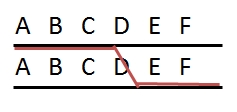
Imagine two genes/markers, G and H, which are both located on the same chromosome. Imagine an individual resulting from a cross between Parent 1 (GGHH) and Parent 2 (gghh). This individual will have received GH from Parent 1 and gh from Parent 2 and thus wil be GgHh. The gametes formed by this individual will be as follows:
NO CROSS-OVER results in gametes GH and gh (both scored as 'parental'), expected to occur in equal proportions.
ONE CROSS-OVER between G/g and H/h results in gametes Gh and gH (both scored as 'recombinant') in equal expected proportions.
TWO CROSS-OVERS between G/g and H/h results in GH and gh gametes. These are also scored as 'parental' or non-recombinant, because only the markers are scored and nothing is observed about the piece of DNA in between the markers.
|
|
Two gametes produced after double cross-over. Generally: odd numbers of cross-overs result in recombinant genotypes, even numbers in non-recombinant genotypes. The occurrence of more than three cross-overs per arm is rare, even for large chromosomes. |
Map distances are estimated by computer programs based on recombination frequencies, estimated from observed genotype frequencies (fractions of individuals that have a certain genotype for a combination of two markers). The larger the true distance between two genes (or markers), the less precise the estimated distance will be, because higher recombination frequencies have higher sampling variance.
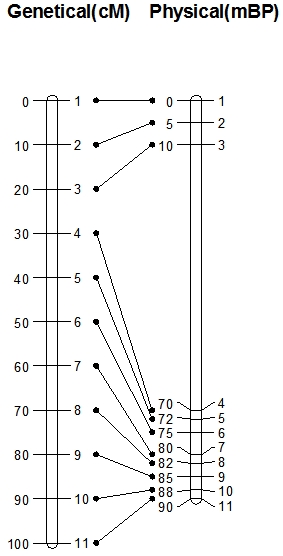 In the picture on the left you see two types of maps: on the left hand side you see a genetic map with 11 evenly spaced markers (1-11). The space between the markers is measured in centiMorgans, which, at short distances (up to about 10 cM) approximately represent the percentage of recombination. The distance between, for example, Marker 1 and Marker 2 is 10 cM, so the percentage of recombination between Marker 1 and Marker 2 is about 10%. Marker 1 and Marker 2 are therefore linked and the large majority of gametes carry the parental combinations of alleles. However, this does not automatically mean that Marker 1 and 2 lie physically closely together on the chromosome! This is visualized in the physical map of the same chromosome on the right hand side. Physical maps are based on the distances expressed in number of base pairs of the DNA. On the physical map in the picture, you see again the positions of Markers 1-11 and their positions, measured in millions of base pairs counted from the top. Marker 1 and Marker 2 are 5 million base pairs apart.
On the genetic map, Markers 2 and 3 are 10 cM apart, and Markers 3 and 4 also. However, on the physical map, we see that the genetic distance does not predict at all the physical distance. Distance between Marker 2 and 3 is about 5 million base pairs, and distance between Marker 3 and 4 is 60 million base pairs. This implies that in the long stretch of DNA between Marker 3 and 4 as many recombinations occur as on the much shorter stretch between Marker 2 and 3. So, per million base pairs, recombination is much lower between markers 3 and 4 than between 2 and 3.
Genetic maps are generated using the pairwise recombination frequencies between markers. Physical maps are generated by sequencing: the order of the DNA base pairs is assessed by sequencing machines and put together. When the sequences of markers used in a genetic map are known, they can be located on the physical map, and their positions may be estimated or determined.
During meiosis, cross-overs can occur, resulting in recombination. As will be seen below, not every crossover will be observed in the progeny. The probabilities of cross-overs occurring are not the same along the chromosome, as illustrated above. Usually fewer cross-overs per million base pairs occur close to the centromere, compared to the regions further away from the centromere. If many cross-overs occur within a short stretch of DNA, this results in a long distance on the genetic map. This region is then called a recombination hot spot. If few cross-overs occur on a long stretch of DNA, this results in a small distance on the genetic map, whereas the physical distance is great. This region is called a recombination cold spot. This explains the large distance between markers 3 and 4 on the physical map compared with the relatively short distance on the genetic map.
Show/hide comprehension question...
|
|
|
|
|
In non-polymorphic DNA regions, recombinations remain unnoticed (top). In the flanking polymorphic regions (A/a and I/i) we may find polymorphic markers to determine recombination frequencies. The (polymorphic) markers closest to the non-polymorphic region and flanking it (A/a and I/i), may recombine frequently, especially when the non-polymorphic region is relatively long. |
In the previous section, we saw that a recombination hot spot can result in relatively large distances in genetic maps. This is caused by many recombinations occurring in a relatively short stretch of DNA (physical map).
When both chromosomes of a diploid plant have an identical stretch of DNA, i.e. no polymorphism there, cross-over events may occur in that region, but this will remain unnoticed in the progeny, since in that region no markers can be developed (picture on the right: top). Still recombinations in that area occur, and will result in recombination between the polymorphic flanking areas (picture on the right: bottom) if there are any. Therefore the non-polymorphic area will result in a gap in the linkage map, since the flanking markers have a rather high percentage of recombination, and no markers occur in between them. If there are non-polymorphic regions at the ends of chromosomes, these will not be represented in the genetic map. Non-polymorphic regions may occur if two parents of the mapping population have one or more DNA fragments in common, because they have a common ancestor. Heterozygous regions are needed to observe recombination events in the resulting progeny.
Alternatively, a DNA fragment may have no homology with the sister chromosome. This may be the case in a introgression from a different, related, species. In such a region, there will be (almost) no chromosome pairing in the meiosis, and hence (almost) no recombination (picture below). This will result in a cold spot. Markers may be developed due to the high polymorphism, but they will cluster on the linkage map, since they are at distances of 0 cM from each other.
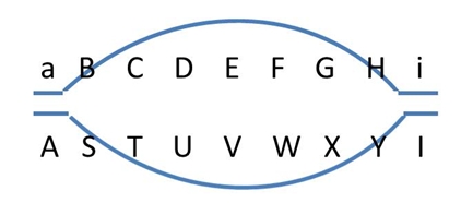
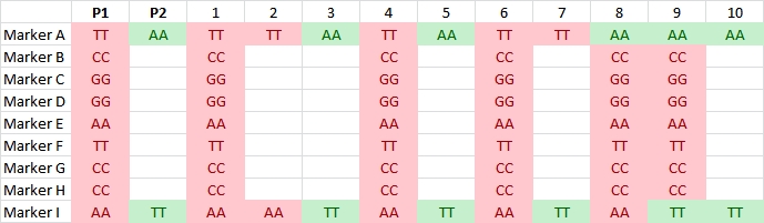
Illustration of two SNP markers segregating in a RIL or DH population (data of 10 individuals shown). They have no corresponding sequence in parent P2. The identical segregation pattern indicates that the two markers are located on the same DNA fragment that probably is not homologous between the two parents.
Summary
→ Genetic maps are expressed in centiMorgan units and are calculated from the pairwise recombination frequencies among markers and/or genes segregating in a progeny
→ Physical maps are expressed in base pair units and generated by sequencing
→ Recombination hot spots are regions on the chromosome (= on the physical map) where relatively many recombinations occur
→ In non-polymorphic DNA regions cross-overs occur, but their effect in terms of recombination may only be noticed in the polymorphic flanking regions of that segment or go unnoticed entirely if there are no polymorphisms
Show/hide comprehension question...
Show/hide comprehension question...
Show/hide comprehension question...
Show/hide comprehension question...
After P. Stam, Modern statistics for the life sciences
Double recombination events
The recombination frequency between two genes/markers is indicated with 'r' (see picture below): 0 < r < 0.5 (diploids). As we have seen before (Linkage, recombinations and map distance), the recombination frequency over the interval A – C (rAC) is less than the sum of rAB and rBC. Thus rAC < rAB + rBC. This is because (rare) double recombination events (a recombination in both A - B and B - C) do not contribute to recombination between A and C. In fact, any even number of recombination events would go unnoticed, whereas any odd number of recombination events could be observed in the progeny.
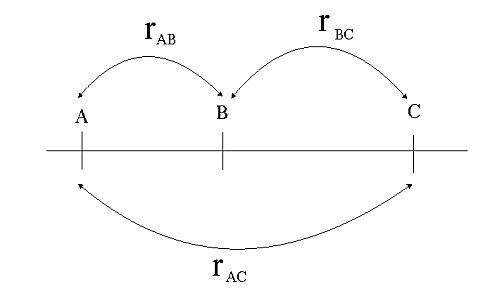
Non-additivity of recombination frequencies: rAC < rAB + rBC.
Double recombinants, i.e. gametes resulting from a recombination event in both the intervals A –B and B – C do not contribute to recombination over the interval A – C.
Theoretically, the most direct way to detect linkage would be to observe the genotypes, and their frequencies, of gametes produced by a parent that is heterozygous at two linked loci (figure below, in which P= parental type of gamete, and R = non-parental, recombinant type of gamete).
Unfortunately, in most plant species, it is not possible to directly assess the genotypes of gametes (an exception are doubled haploids, which reflect the gametic constitution, or testcross/backcross situations). Therefore, we often have to resort to indirect ways of observation, which means not observing individual gametes but the result of fused gametes, i.e. the offspring of two parents. In practice, linkage of loci is derived from the observation that among the offspring, alleles are associated ('go together more often than expected by chance') rather than segregating independently. With co-dominant markers, like SNPs, such an analysis is sometimes, but not always, straightforward, since recombinant and non-recombinant genotype classes can be distinguished. With dominant markers, gamete genotypes and their frequencies can still be determined unambiguously in terms of being caused by recombinant or non-recombinant gametes in a DH, testcross or backcross:
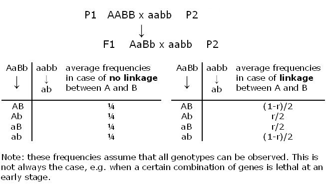
The backcross described above is the most simple in this respect, since the frequencies of recombinant and non-recombinant gametes can be obtained by simply counting the numbers of individuals in the recombinant and non-recombinant genotype classes. In many other cases, there is not such a one-to-one relation between marker genotype class and the origin (non-recombinant or recombinant) of the gametes that gave rise to this phenotype. For example, even for codominant markers, in an F2, the double heterozygous class AaBb is ambiguous: individuals in this class could be from two non-recombinant gametes (AB with ab) or from two recombinant gametes (Ab with aB), so that this class cannot be counted as entirely doubly recombinant or non-recombinant. The situation of not being able to count the recombinant and non-recombinant gametes exactly often also arises for dominant markers, or simply because of missing scores for one or both markers.
Assume the observed recombination frequencies in the picture below:
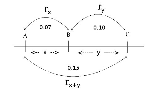
Ordering genes on the basis of observed recombination frequencies. The order A – B – C is readily inferred. When many loci are to be assembled into a linkage map, ordering requires 'smart' computerization, since the number of
possible orders increases approximately exponentially with the number of loci.
The distance 'x' between markers A and B is estimated by recombination frequency rx (and y by ry). The closer A and B are together, the smaller the expected recombination frequency between A and B: rx. Note that the recombination frequency between A and C (rx+y= 0.15) is smaller than the sum of rx (0.07) and ry (0.10) due to double recombinations between A and C. In fact, any even number of recombination events would go unnoticed, whereas any odd number of recombination events could be observed in the progeny.
Assuming no interference
In the absence of interference, recombination events in adjacent intervals (and as a result, in any pair of intervals) are independent. Under the assumption of no interference:
rx+y = rx(1 - ry) + (1 - rx)ry = rx + ry - 2rxry
(where:
rx = the recombination frequency between loci A and B
ry = the recombination frequency between loci B and C
rx+y=the recombination frequency between loci A and C)
In the example the expected recombination frequency between A and C, as estimated from AB and BC, would then be 0.07 + 0.10 - 2*0.07*0.10 = 0.17 - 0.014 = 0.156, close to the 0.15 that was observed from the genotype counts for the A and C locus directly.
Assuming positive interference
A consequence of positive interference (smaller chance on cross-overs in the neighborhood of an existing cross-over) is:
rx+ y > rx + ry - 2rxry.
Genetic mapping functions
A genetic mapping function describes the mathematical relation between recombination frequency (r) and map distance (x). The map distance between two loci is the average number of recombination events per meiosis between those loci. The exact relation between r and x depends on the degree of interference between recombination events, in adjacent intervals.
|
|
Extra information (for illustration only): The most widely used mapping functions, Haldane's (H) and Kosambi's (K) mapping functions Haldane's mapping function (derivation not shown here) uses the assumption of no interference and reads: r = ½ (1-e-2x). Kosambi's mapping function is a mapping function that (empirically) appears to be fairly well describing the strength of interference in many organisms. It reads: r = ½ tanh(2x). This results in (derivation not shown here):
Note that Kosambi's leads to a shorter map distance for a given recombination frequency. In addition to these two mapping functions a whole family of genetic mapping functions has been designed, each corresponding to a given degree of interference (after Stam, Study guide from the Wageningen University MSc course Modern statistics for the life sciences). Note also that Haldane and Kosambi are non-linear functions.
|
Summary
→ Recombination frequencies are non-additive. Map distances (in cM units) are
→ Recombination can be reduced or enhanced by recombination events in adjacent intervals: interference
→ Mapping functions describe the mathematical relation between recombination frequency and map distance
→ Haldane's mapping function uses the assumption of no interference; Kosambi's mapping function allows for positive crossover interference. Many other mapping functions exist. They do not result in big differences, especially not for small distances.
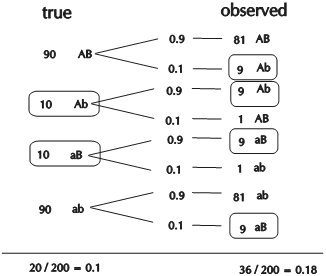 (after Stam, Study guide of the Wageningen University MSc course Modern statistics for the life sciences)
Errors in genotype scoring, or genotype classification, will lead to incorrect estimates of recombination frequencies, and hence, incorrect genetic distances. We illustrate this effect by means of a simple numerical example. Suppose the following situation:
In reality, there would be 20 recombinants (blue+smooth and red+wrinkled) out of 200 pollen grains (figure, left). From the score, it appears that 36 out of 200 would be recombinants
(figure, right). So, in case of 10% erroneous scoring, the estimate of r (0.18) is almost twice as large as the real value! It should be noted that when recombinants are incorrectly scored as non-recombinants, the recombination frequency estimate would actually decrease instead of increase. However, as in the example, if the error scoring is independent of the true genotype, and there are fewer recombinants than non-recombinants (by definition), the non-recombinants would be affected more than the recombinants: in this example, from the 180 true non-recombinants, 18 are now counted as recombinants. From the 20 true recombinants, 2 are now counted as non-recombinants, so this results in a net balance of 16 extra recombinants on a total of 200 individuals.
Similar deviations in calculated distances occur when marker alleles are erroneously scored.
Show/hide comprehension question...
Summary
→ Errors in genotype scoring result in relatively large errors in estimates of recombination frequencies (= overestimations) and map distances
Show/hide comprehension question...
Linkage is deduced from the observation that loci are associated in offspring and not segregating independently. As we know, the process involves the following steps:
Assume an autogamous species, using SNP markers:
In this example we have scored the parents and progeny for 12 SNPs. Four of them are not polymorphic (3, 5, 8 and 11):
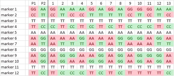
We identify the parental origin of each SNP allele, and color accordingly red (origin P1) or green (P2). Next we convert the P1-alleles to A, and the P2-alleles to B, and delete the non-polymorphic SNPs:
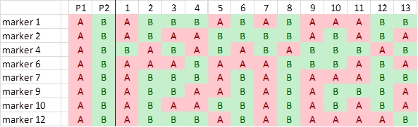
Comparison of segregation patterns show that highlighted markers 1, 7 and 12 show an associated segregation pattern. There is only one recombination:
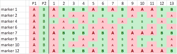
This indicates that markers 1 and 7 are more closely linked with each other than with marker 12.
The chromosomes below illustrate the position of markers 1 and 7 relative to marker 12. Note that we do not know the orientation of the markers yet.
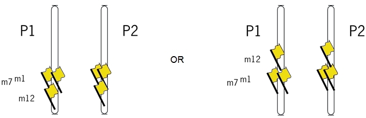
Suppose, we find an additional marker (13) that has segregation pattern which is similar as that of markers 1, 7, and 12, but there is one additional recombination event in this set of 13 progeny plants: plant 1, relative to markers 1, 7 and 12:
The numbers of recombination events represented by this set of progeny is presented in the table below:
|
|
marker 7 |
marker 12 |
marker 13 |
|---|---|---|---|
|
marker 1 |
0 |
1 |
2 |
|
marker 12 |
1 |
- |
1 |
|
marker 13 |
2 |
1 |
- |
So, logically, markers 1 and 7 are closer to marker 12 than to marker 13:
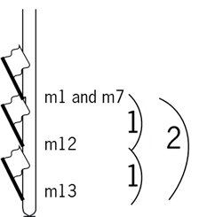
Now we find another pair of markers that has an associated segregation pattern: markers 2 and 10. Their pattern is not associated to the pattern of markers 1, 7, 12 and 13, so they form a different "linkage group". Linkage between markers 2 and 10 is not absolute, since there is recombination (plant 7):
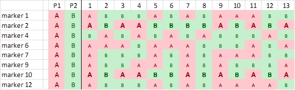
Etcetera. Finding associations between numerous markers in a large number of individuals is an automated process.
After P. Stam, Study Guide of the Wageningen University MSc course Modern statistics for the life sciences.
The outcome of a mapping experiment depends on the composition and size of the sample population. The larger the mapping population, the more confidence we have in the estimates of recombination frequencies and map distances. For most purposes populations of size in the range 80-400 are used. Of course the quality of the marker scores is a major issue as well.
A map that is based on a mapping population of 100 RILs will result in a (slightly) different map than a map calculated on 100 different RILs derived from the same cross. Just because of the fact that every population is the result of sampling gametes, a non-deterministic procedure, recombinations may occur more frequently in one set of 100 individuals than in another set of 100 individuals. The figure below shows the simulated result of replicate sampling of an F2 population and the best map corresponding to each sample. Although the variation between these maps with respect to marker order is nil, the resulting total map length as well as the inter-marker distances are quite variable. This demonstrates that the 'ultimate true map' does not exist. A calculated map is the best statistical approximation, given the sample population.
|
|
Graphical representation of ten linkage maps, derived from one true map by simulation (not treated in detail). For each of these maps, a data set was generated by stochastic simulation. The true map (length 100 cM) on the left corresponds to the recombination rates between adjacent markers used in the simulation. For each of these maps, different data sets were generated, using the recombination rates. Due to the variation in the sample composition, the resulting maps are different. Notice that for a given marker pair the estimated map distance may vary considerably (see lines connecting marker pairs between maps). If, in addition to sampling variation, there would also be errors and missing values, in the population for some markers, the differences between the maps will be larger and there might also be reversal of marker orders between different 'replicate maps'. |
A linkage map based on another population will yield a map with larger differences: also the apparent order of some markers may have changed. This will be explained later.
Summary
→ The linkage map may vary depending on the composition of the sample population.
Show/hide comprehension question...