Markers
Marker-Assisted Selection
Breeders want to improve their crops for many traits: yield, fruit taste, resistance to pathogens, processing quality (e.g. bread baking in wheat), tolerance to drought, etc. Many of these traits are quantitative, i.e. they are varying along a continuous distribution from low to high trait values. Only few characters are qualitative, i.e. they can be scored as discrete values or in clearly distinct classes such as white versus red flowers. Some of these, like for example monogenic resistances, may still require special phenotyping trials to score, for every individual in a population, the genotype.
Quantitative traits often are determined by several to many genes, each with a possibly small effect on the trait value. In addition to the genetic effects, the environment may add to the variation that we observe in the quantitative trait values. Consequently, phenotype does not directly reflect the genotype. A further difficulty is that many quantitative traits cannot be evaluated well on single plants, but should be measured on a larger number of plants of every genotype. For example, in wheat, yield and bread-baking quality cannot be measured on the basis of single plants. Also, bread-baking quality is a rather cumbersome trait to evaluate, requiring expensive analysis in the laboratory.
All these complications make it an attractive idea for the breeder to select directly for the presence of favorable genes and against unfavorable genes, instead of on the basis of test results for quantitative traits. What the breeder would really want is to be able to directly select the genotype, but for many traits they can only observe the phenotype and even then it may require considerable costs, time and effort. "Marker-assisted selection" (MAS) is the strategy that aims at replacing phenotypic selection or complementing phenotypic selection with selection based on genotype as established from the DNA sequence in the region of a gene of interest.
Molecular markers have additional advantages, as will be shown in more detail later: they can be used for early selection, off-season and off-location seleection, they can speed up the selection process, they can allow more seedlings to be evaluated, and they can even be used to select for phenotypic traits that are not or cannot be measured (e.g. a disease resistance in the absence of the disease itself) or to enable combining multiple genes that based on the phenotype could not be distinguished individually. They can also help in finding the exact location of functional genes in order to enable cloning of these genes and they help to understand the genetic basis of many traits.
Authors of this module are lecturers of the chair groups Plant Breeding and Nematology of Wageningen University, the Netherlands:
Dr. J.C. Goud, Dr. R.E. Niks, Dr. Chris Maliepaard, and Ir. H. Thiewes.
Part of the content of this module is roughly based on the following scientific article:
B.C.Y. Collard, M.Z.Z. Jahufer, J.B. Brouwer & E.C.K. Pang (2005) An introduction to markers, quantitative trait loci (QTL) mapping and marker-assisted selection for crop improvement: The basic concepts. Euphytica (2005) 142: 169–196.
Arrangements have been made with Springer publishers and with the first author to use the text. However, the text in this module has been changed considerably from the original text in the article.
Chromosomes are very long (double) strands of DNA bases (DNA nucleotides). The bases of one strand correspond with counterpart bases on the other strand, and are called "base-pairs", often abbreviated as bp. The identity of the linearly arranged base pairs is called the DNA sequence. The base pairs together make a "story", based on an alphabet of only 4 letters (A, C, G, and T). A relatively small proportion of the chromosome consists of sequences that are expressed, and therefore contribute to the life function and appearance of the organism. The function of a large proportion of the DNA (formerly indicated as "junk DNA") is not yet fully understood. However, the sequences that are not expressed may still contribute to the function and appearance of the organism in some way. Within each species, and even between species, a lot of the DNA sequences are conserved (nearly identical), but also a lot is variable. The level of conservation is often sufficient to know which chromosome in one individual is equivalent (homologous) to which chromosome of another individual. However, between such homologous chromosome pairs, more or less variation in DNA sequence can be found. At the place (technically called "locus") of the gene for flower color, one chromosome may carry the allele for red flowers, the other for white flowers. The alleles at this locus hence will have a (somewhat) different DNA sequence. Between species there may also be larger structural rearrangements of (parts of) chromosomes. A whole set of tools has been developed to visualize variation in DNA sequence between homologous chromosome regions. A visualized difference in DNA sequence can be used as a "marker", to indicate ("mark") that region of the DNA strand. In principle for the whole genome (all DNA of the nucleus together) markers may be developed, both inside and outside genes.
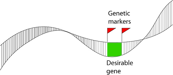
If a certain marker happens to be located near a gene for a useful trait, this marker may be of interest to the breeder. In case the gene that is near the marker occurs as one (favorable, for example resistance) allele on the chromosome of one parent (homozygous for that allele) and as a different (less favorable, for example susceptible) allele on the chromosome of the other parent, the marker (= visualized difference of a nearby DNA sequence) may be used to know which of the segregating progeny of a cross of these two parents has the one allele of the gene, and which the other, and hence which of the progeny to select. Also when the association between marker and gene is high (but maybe not exactly 100%), it may still be useful as a fast and cheap way to screen for resistance without the need of phenotyping the resistance of the plants.
The distance between the sequence on which the marker is based and the gene of interest is relevant. The larger the distance between the marker locus and the locus of the gene of interest, the larger the chance that the chromosomes during meiosis perform a "crossover" between the loci. When the plant is heterozygous for both the marker and the gene, the gamete in which such a cross-over occurred in between the two loci, will show a "recombination": the marker allele that was linked to the favorable allele of the gene gets connected with the marker that indicated the unfavorable allele, or the marker that was linked to the unfavorable allele gets associated with the marker that indicated the favorable allele. The larger the distance between the marker locus and the locus of interest, the less reliable the association between the marker and the trait gene in inheritance is. This is because of the increased probability of recombination between the marker locus and the gene.
Summary
→ Genetic markers are useful for MAS when they are linked to genes of interest
→ The larger the distance between the marker locus and the locus of interest, the higher the chance of recombinations and thus the less reliable the association between the marker and the trait gene is
Genetic markers can be divided into three types:
Morphological markers are the first markers that were used in plant breeding. They are visible in the phenotype of an individual organism. When the trait of interest is located closely to the locus of the morphological marker, this marker can be used for MAS. In any parental pair, used in a crossing, we can only use the morphological traits for which these two parents differ. This may be hairiness of leaf base, color of flower, some leaf shape aspect, leaf tip necrosis etc. However, such morphological markers do not usually cover the entire genome, which limits their use. Besides, in modern cultivars, the morphological aspects that differ between pairs of cultivars is very limited, and hence the number of possible morphological markers is also very limited. Further, several of such markers can only be judged in advanced stages of plant development, e.g. flower colour. So, an early and rapid screening (i.e. in the seedling stage) is not possible, since we should wait until the population to be judged is flowering in order to use flower color as a marker.
Biochemical markers are allelic variations of enzymes, called isozymes. Different isozymes of a specific enzyme have the same function in an organism. Isozymes differ slightly in structure (size, electrical charge, three-dimensional structure) which cause them to move at a different speed through an electrophoresis gel. These detectable differences are the basis for biochemical markers. Just as morphological markers, different isozymes can be used to select for desired traits if they are linked to genes of interest.
For biochemical markers, the choice is also limited. There is no infinite number of enzyme systems, and for each enzyme system, the parental pair should be checked whether they have in any of their organs and development stages different isozymes. Each isozyme scoring requires a separate analysis. So, although the number of potential biochemical markers is much larger than morphological markers, their application is cumbersome and it is hard to find enough biochemical markers to cover the whole genome of the plant. Since the development of DNA-based markers, they are hardly used anymore.
DNA-based ("molecular") markers to be applied for selection in a population derived from a cross between two parents are based on variation in sequences in DNA. For example, for a cross of two homozygous parents, it is based on variation between alleles of one parent versus those of the other parent. For a cross where one or both parents are heterozygous, it is based on variation between the two alleles within the same parent(s).
Even small differences in DNA sequence may be visualized to become a marker. Since the DNA consists of a huge amount of DNA base pairs, within most crops a great amount of variation accumulated over time. Most of the first generation DNA markers appeared in non-coding regions of DNA, which are selectively neutral areas of DNA. Nowadays, the aim has shifted to markers that are based on DNA sequence differences inside genes. Since all DNA variation inside and outside genes can be used to develop a marker, the number of DNA markers that can be developed is in principle almost infinite, as long as there is variability across different genotypes at many places in the genome.
An additional advantage of DNA markers is that DNA occurs in each plant cell, and all plant cells (in principle) of an individual carry the same DNA. So, any plant cell or tissue is as good as the other to extract DNA, and we do not have to wait until plants developed to maturity before we can isolate DNA to visualize the markers. Use of DNA markers does have limitations as well. These will be discussed later on.
Development of DNA markers
DNA markers are visualizations of sequence differences in the DNA. These visualizations can be realized in different ways. The older marker types were developed using various tools and principles. Often, the different procedures involve techniques such as:
With DNA sequencing techniques becoming increasingly efficient and inexpensive, it is relatively easy to find large numbers of SNPs: single nucleotide polymorphisms. This marker type is based on differences of only one base pair between parents.
|
3'TGAACTAGTACCAAGGAT 3'TGAACTGGTACCAAGGAT |
DNA of a genotype that is heterozygous for a C/T SNP polymorphism, highlighted in red. The SNP is called after the forward DNA strand base (5' strand).
High throughput sequencing methods now allow the generation of many DNA sequence fragments. Several software programs have been developed to compare the generated sequences ('reads') across a number of accessions and to find SNPs that are polymorphic between accessions. Even for species of which no reference genome is available, this sequencing and the selection of SNPs can be done.
Effect of developmental stage
Many traits, such as fruit size, become visible only at a certain developmental stage. However, the genes for fruit size (and DNA markers associated with these genes) are already present from the moment of fertilization. As soon as the plant is big enough to harvest a part of the plant (a small leaf will be enough), one can screen the plant material for selected parts of the DNA. The independence of developmental stage is an important advantage of molecular markers above morphological markers.
Summary
→ Three different types of genetic markers exist: those that are detected morphologically, biochemically or by DNA analysis
→ Each type of genetic marker is analyzed visually; only the visualization method used differs
→ DNA markers exist in almost infinite numbers, they are not affected by the environment, and they can be determined in any developmental stage
DNA markers are useful if they reveal genetic differences between two individuals. These markers are called polymorphic markers, while markers that do not discriminate are called monomorphic markers (figure below). When a marker is polymorphic in a certain population, it can be used for selection within this population. However, a marker that is polymorphic in one population, might be monomorphic in another population and thus be useless there. Different forms of a DNA marker are called marker alleles.
|
|
|
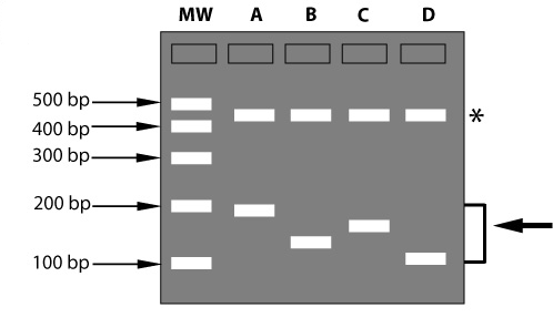
Example of a monomorphic and a polymorphic DNA marker. Some types of DNA markers are made visible as bands on gels. MW: molecular weight DNA ladder, used to estimate the sizes of the DNA fragments. The shorter a fragment, the faster it moves through a gel and the further it has advanced from the gel slots at the top. bp: sizes of DNA fragments are measured in base pairs. The gel picture shows a monomorphic DNA marker (indicated by an asterisk) and a polymorphic DNA marker (indicated by the arrow on the right) in genotypes A, B, C and D. It depends on the population tested whether a marker is monomorphic or polymorphic: in case there is another genotype E, the marker indicated with an asterisk might show a band at a different place. Then this marker is polymorphic. |
Historically, several types of DNA markers have been developed, introduced and applied. Most markers needed DNA amplication by PCR and separation on a gel. Methods to detect and visualize markers differed, leading to marker types as RAPD, RFLP, AFLP, SSR, CAPS and SNP markers. All of them had their advantages and disadvantages. Aspects considered to value a marker type include:
Since most markers have been replaced by SNP markers now, and the others became more or less obsolete, we will not explain the methodology of all the marker types. One genetic property, however, will be explained: dominance/co-dominance of markers. This is a very important aspect to take into account when a breeder applies molecular markers.
When DNA markers of plant accessions are polymorphic, the polymorphism can be observed in two ways:
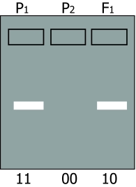
In situation 1, (presence or absence of an amplification product) presence of the amplification product is caused by an allele often indicated as '1'; absence by allele '0',(null-allele). The diploid homozygote 11 results in a band; the homozygote 00 results in no band; the heterozygote 10 results in an amplification product (and a band) which is identical to the product formed by parent 11 (figure below, left). Inheritance resembles that of a dominant trait. Therefore, it is called a dominant marker.
An essential aspect of dominance is that the heterozygote cannot be distinguished from one of the homozygoes, but that the other homozygote can still be distinguished from these two. In the case of codominance the heterozygote and the two homozygotes can all be distinguished from each other.
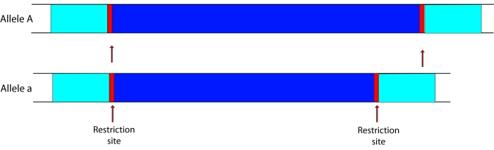
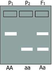
In situation 2, two types of bands are formed by fragments of different length: Parent 1 is homozygous and has AA alleles (alleles for long fragment) and parent 2 has aa (alleles for short fragment). The heterozygous offspring is Aa, so it has the alleles for both the long and for the short fragment, resulting in two bands on the gel.
In this case, the heterozygote and both homozygotes can all be distinguished from each other. This marker is called a codominant marker (Figure below, right).
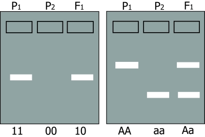
Comparison between dominant (left) and codominant (right) markers. Codominant markers can clearly discriminate between homozygotes and heterozygotes, whereas dominant markers do not. Genotypes at two marker loci (1 and A) are indicated below the gel diagrams.
For the dominant marker, locus 1 may carry two 1-alleles (1-1, or 11), two 0-alleles (0-0, or 00), or - in the heterozygote - one 1-allele and one 0-allele (1-0, or 10). In this example, the 0-allele results in absence of a band, for example caused by absence of an amplification product. Allele 1 results in presence of an amplification product and thus a band, regardless of the number of 1-alleles (one or two). Therefore, the heterozygote 10 and the homozygote 11 cannot be distinguished. For the co-dominant marker, allele A and allele a each result in a product, which is of different size, so the heterozygote can be distinguished from each of the homozygotes.
Some techniques that visualize variation in DNA sequences result predominantly in dominant markers; others in co-dominant markers. That depends on the strategy that is followed and on the nature of the sequence variation between the parents.
|
Dominant alleles of trait genes versus dominant alleles of markers In Mendelian genetics, dominant alleles of genes that code for traits overrule the effect of recessive alleles present. For example: if B is the dominant allele for hairy leaves and b is the recessive allele for smooth leaves, both BB and Bb plants have hairy leaves and bb plants have smooth leaves. In dominant markers, only dominant alleles can be detected as a band. So, on the gel, we see either a band or no band. Alleles that result in absence of a band are null-alleles: no band is formed, because the DNA fragment did not amplify. This could be caused by a number of different reasons. Therefore, in different individuals, different null-alleles might be present. Dominant markers are then sometimes coded as B_ versus bb). SNP markers are read in terms of the base pair that is involved: A, T, G or C. In the example in the picture on SNPs, the parents may be T, and G, respectively. SNP markers are co-dominant: if one chromosome carries the base pair AT and the other GC, (heterozygous), the marker is written as T/C. Note that also in genes that influence traits more than two alleles are often present. DNA-sequencing of genes has shown that in by far most genes, DNA polymorphism exist at population level. Some of those DNA differences may lead to a different trait expression, others are phenotypically neutral. Each of the DNA- sequence types may be considered a different allele. Also note that in the F1 of a cross of a cross pollinated species, e.g. apple, where both parents may be heterozygous, possibly for different alleles, more than two alleles (of a marker or a gene) may be segregating (B1B2 x B3B4) and there are different heterozygotes in the progeny that may or may not be distinguishable. In practical use, SNPs are biallelic, they allow just two variants to be visualized. |
Summary
→ Polymorphic markers indicate genotypic differences between the individuals tested.
→ It depends on the population tested whether a marker is monomorphic or polymorphic.
→ Co-dominant markers can discriminate between homozygotes and heterozygotes.
→ Dominant markers visualize only the presence/absence of a single marker allele and therefore do not allow a heterozygote for that allele to be distinguished from the homozygote for that allele.
→ The absent band in dominant markers represents a null-allele.
I want an alternative explanation | Move on to: Types of DNA markers
If a marker in a population has only one form, it cannot be used for selection. It is called a monomorphic marker. A polymorphic genetic marker can be useful for selection, when it is linked to a gene for a desirable trait.
We will now show three forms of DNA markers:
Monomorphic markers
|
|
|
|
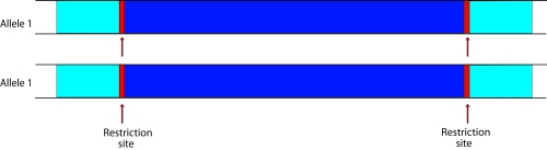
Top figure: if all tested individuals have the same allele, there is no polymorphism. The marker is a monomorphic marker (450 bp bands indicated with an asterisk). It does not reveal differences in alleles, and cannot be used for genetics or selection in breeding. Lower figure: allele 1 is present in all individuals tested. The part of the DNA between the restriction sites (red) can be made visible on a gel, using a so-called probe: a labeled DNA fragment that binds to specific DNA sequences and in that way 'stains' the DNA fragment.
Polymorphic markers which are dominant
|
|
|
In a dominant polymorphic marker only one allele can be made visible. Let us assume that the procedure to make the marker visible involves:
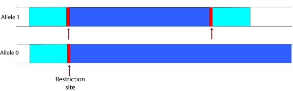
Allele 1 results in a visible band on the gel. In allele 0 one restriction site is missing. The next restriction site could be too far away, resulting in a fragment that is too long to amplify. In case of a homozygote carrying allele 1 (11), or a heterozygote 10, a band will appear on the gel. In case of a homozygote carrying allele 0 (00), no band will appear on the gel.
Polymorphic markers which are codominant
|
|
|
Codominant markers. For simplicity, we use here only two alleles: A and a (The gel on the right shows AA and aa parents and an Aa F1 An F2 population would give a segregation of all three patterns..
Codominant markers can discriminate between all possible gene combinations. Both alleles anneal to the same type of stained DNA probe, which is used to visualise the fragments as a band on a gel. The probe anneals to a specific region in the fragment. Outside the probe region, allele A has more sequence repeats than allele a. Because allele A is bigger than allele a, allele A will travel slower through an electrophoresis gel. A homozygote for allele A (so AA) will have one band (in fact two times the same (A+A) band). A homozygote for allele a (aa) will also have one band but this band will have moved faster (lower on the picture) than the band of allele A. Since a heterozygote (Aa) has a copy of allele A and a copy of allele a, a heterozygote will have both bands.
Show/hide comprehension question...
DNA markers are formed by different types of variation in the nucleotide sequence. The most important are substitutions (point mutations: substitution of one nucleotide by a different one), rearrangements (insertion or deletion of nucleotides, also called 'indels') or errors in replication, such as duplications.
These variations can be detected by different technical methods. Those printed in red are treated in more detail below; the rest are not part of the course, but you can come across them in older literature:
Of these, SNPs and SSRs are currently the most used. Through the growing use of sequencing techniques, techniques that decipher the DNA genetic code, numerous SNPs can be discovered. Because of this and the availability of high-throughput scoring of many SNPs for many individuals at the same time, SNPs are currently very important as markers. SNPs have the additional advantage that they can be detected in the alleles of genes.
Because of the sequencing technologies becoming cheaper and more high-throughput all the time, the scoring of SNPs by using SNP arrays or bead based technologies, will be complemented or replaced by technologies generating, in segregating populations, for every individual in the population, smaller or longer sequence reads of segments of DNA containing more than a single SNP and that these reads are then used as multi-SNP sequence markers. These approaches are called genotyping-by-sequencing (GBS).
|
|
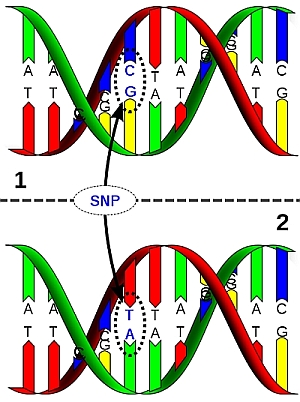
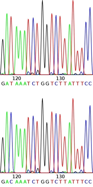
DNA sequences of homologous chromosome regions can be determined and compared between members of the population of the species. The sequence is often conserved: that means that the base sequence is almost identical between the individuals. This is in particularly true for genes (coding regions) and less so for non-coding regions. Comparison of conserved base sequences between individuals may reveal that they differ for only one base pair (nucleotide) in a stretch of DNA. This is called a Single Nucleotide Polymorphism (SNP, pronounce as "snip"). Such a polymorphism can be visualized as follows (figure below): During sequencing, the nucleotide sequence of a stretch of DNA is determined. Depending on the sequencing technique used (not treated here), this is observed as peaks of different colors (see example in figure), bars, or spots, representing the nucleotides in the DNA. The whole process is highly automated, e.g. peaks are read by special cameras and analyzed directly by a computer. SNP markers are often based on coding regions, since those are relatively conserved. SNPs that occur in the gene of interest itself (instead of on some gene that happens to be linked to the gene of interest), are the ideal marker to be used in marker-assisted selection. The association between the SNP allele and the allele of interest cannot be disturbed by a rare recombination event (although recombination within a gene is not impossible, but very unlikely). When SNPs occur in a gene, they do not always alter the function of the gene, since different codons may encode the same aminoacid. A change in base pair that does NOT alter the aminoacid that is coded for is called a 'synonymous mutation'. A base pair change that leads to a different amino acid is called a 'non-synonymous mutation'. Not all aminoacid changes change the properties and function of a protein. So, many DNA variations are phenotypically neutral.
Both alleles can be made visible, so SNPs are codominant markers. |
|
DNA molecule 1 differs from DNA molecule 2 at a single base-pair location (a C/T polymorphism). |
 High-throughput SNP detection using sequencing techniques.
After identification of SNPs between the parents, the breeder may run many individuals in the progeny for such a SNP of interest. Such work is usually outsourced to specialized companies. The high-throughput running of SNPs needs knowledge of the DNA sequences flanking the SNP (that should not be polymorphic) and the bases that constitute the SNP. In this application we may run thousands of individuals for a certain SNP at relatively low cost.
There are also SNP platforms (spotted on chips, arrays), in which thousands of different SNPs may be run on individual DNA samples. In that case relatively few DNA samples are run against so many SNPs that a genome covering data set is obtained (about 100 € per DNA sample).For barley, for example, a set of 9000 SNP markers is available (the '9k Illumina Infinium iSELECT chip'). For each pair of barley cultivars, 2500 - 3000 of these SNPs are typically polymorphic.
Show/hide comprehension question...
Summary
→ SNPs are codominant markers
→ They occur relatively often, sometimes even within functional genes
→ SNPs are mostly detected by sequencing techniques
→ For a given SNP many plants can be screened efficiently by high-throughput techniques.
I want an alternative explanation | Move on to: SCAR
A SNP is a small genetic difference, consisting of one nucleotide (base pair). For example, a SNP occurs when a DNA sequence AGGGTTA is altered by a mutation to ATGGTTA. This mutation may have occurred recently, or many generations before.
Sequence Characterized Amplified Regions (SCARs) uses the sequence of polymorphic fragments of DNA, such as sequenced fragments that are picked-up from mRNA. The primers that are used for SCAR are not chosen randomly but they are especially developed to amplify a unique site in the genome. The primers are about 15-30 nucleotides. Such long primers will fit only one specific DNA sequence in the organism, and are very unlikely to fit by chance some non-target DNA sequence in the genome. Because of their length that corresponds to a sequence in the genome, DNA fragments are reliably amplified and reproducibly generated independent of the lab that runs those markers.
The procedure is as follows:
Dominant or co-dominant. The polymorphism displayed by SCAR markers may consist of amplification of DNA in one parent and failure in the other parent. Such a polymorphism leads to a dominant SCAR marker. A second possibility may be that in both parents an amplified DNA fragment is obtained, but of different size. In that case we have obtained a co-dominant marker. Finally, in both parents an equally long DNA fragment may appear from the PCR. Then a further possibility to find and exploit polymorphism might be to sequence the obtained fragments and compare the sequences between the parents. For example, sequencing may reveal polymorphism in the 200th base-pair (one nucleotide change). This constitutes a SNP, and may be exploited as explained earlier (see SNP markers).
Summary
→ SCAR markers can either be dominant or codominant
→ SCAR primers are specifically designed based on the sequence of a known DNA fragment
→ SCAR markers are highly reproducible
Simple sequence repeats (SSRs) are clusters of 2-5 nucleotides that are repeated after one another for 10-100 times. These non-coding repeats are present at vast numbers throughout eukaryotic genomes. SSRs consist of dinucleotides, like (CA)n, trinucleotides, like (CAG)n, and tetranucleotides, like (CATG)n, etc. The symbol n represents the number of repeats within a SSR. Polymorphism exists when n has a different value between homologous alleles.
Consider two small pieces of homologous chromosomes with 'caca repeats' (CA)14 and (CA)16. In one homologue, the sequence CA is repeated fourteen times (n=14) and in the other sixteen times (n=16):
CGGCTTTCGCACACACACACACACACACACACACACATTCGGCTCAGCT
GCCGAAAGCGTGTGTGTGTGTGTGTGTGTGTGTGTGTAAGCCGAGTCGA
CGGCTTTCGCACACACACACACACACACACACACACACACATTCGGCTCAGCT
GCCGAAAGCGTGTGTGTGTGTGTGTGTGTGTGTGTGTGTGTAAGCCGAGTCGA
The development of SSR markers starts with the creation of a small genomic library. The genomic library is screened for SSRs using a number of repetitive sequence oligonucleotide (random) probes, to identify desired DNA fragments. The SSRs and their unique flanking regions are then sequenced. Primers are chosen that match the flanking DNA sequence of the SSRs, followed by PCR amplification, after which the DNA is run through a gel. After treatment with ethidium bromide, bands are visible. If the bands are different in size, the amplified fragments ('amplicons') are polymorphic, due to a different number of copies of the repeated sequence.
SSR markers are codominant. In a given population, usually a large number of alleles are detected, because of the large variation in n. SSR markers can be used to analyze closely-related populations within a species, and sometimes even among related species, because of the presence of identical conserved sequences flanking the SSR. Be aware that differences in size between alleles, may favor the amplification of one allele above the other.
Summary
→ SSR markers are codominant and usually detect many alleles
→ SSR markers are highly reproducible
→ SSR markers developed for one species can often also be used in other related species
I want an alternative explanation | Move on to: Characteristics of some types of DNA marker
Throughout the genome, sequences exist that are repeated many times. Simple sequence repeats (SSRs) consist of related elements that each are less than 6 base pairs long. The number of times that they are repeated can differ between alleles on homologous chromosomes. Different alleles can be formed as a result of errors in pairing of the DNA strands, due to the repeated sequences.
Examples of different alleles:
CGGCTTTCGTATATATATATATATATATATTCGGCTCAGT
GCCGAAAGCATATATATATATATATATATAAGCCGAGTCA
CGGCTTTCGTATATATATATATATATATATATTCGGCTCAGT
GCCGAAAGCATATATATATATATATATATATAAGCCGAGTCA
CGGCTTTCGTATATATATATATATATATATATATTCGGCTCAGT
GCCGAAAGCATATATATATATATATATATATATAAGCCGAGTCA
CGGCTTTCGTATATATATATATATATATATATATATTCGGCTCAGT
GCCGAAAGCATATATATATATATATATATATATATAAGCCGAGTCA
CGGCTTTCGTATATATATATATATATATATATATATATTCGGCTCAGT
GCCGAAAGCATATATATATATATATATATATATATATAAGCCGAGTCA
CGGCTTTCGTATATATATATATATATATATATATATATATTCGGCTCAGT
GCCGAAAGCATATATATATATATATATATATATATATATAAGCCGAGTCA
|
SNPs |
SCAR |
SSR |
|
|---|---|---|---|
|
Principle |
Observation in sequencing data |
Amplification with sequence specific primers |
Amplification with sequence specific primers |
|
Type of polymorphism |
Single base changes |
Single base changes, insertions, deletions |
Number of repeats |
|
Level of polymorphism |
High |
High |
High |
|
Dominance |
Co-dominant |
Dominant or codominant |
Co-dominant |
|
Amount of DNA required |
<1-20 µg, depending on sequencing method used |
25 ng/reaction |
25 - 35 ng/reaction |
|
Amount fresh leaf tissue required |
<1 - 20 mg |
25 µg/ reaction |
25 - 35 µg/reaction |
|
Quality of DNA required |
Depending on sequencing method used |
Low |
Medium |
|
Sequence information obtained |
Yes |
Yes |
Yes |
|
Radioactive detection required |
No |
No |
Yes/no |
|
Development |
Sequencing: complex SNPs themselves: easy; they are observed during sequencing |
Complex |
Complex |
|
Cost |
Medium, decreasing rapidly |
Low |
High |
|
Complexity of steps involved |
High |
Low |
Medium/high |
|
Initial costs |
High |
Medium |
Medium/high |
|
Application time |
Fast |
Fast |
Fast |
|
Reproducibility |
High |
High |
High |
More information (optional) on markers can be obtained from Semagn et al.(2006) African Journal of Biotechnology 5: 2540-2568 (link).
Earlier we explained the development of markers. More and more of these markers are published in literature, including the sequences that should be used for the primers. Such published markers can be tested in the lab, whether they work well in the material of interest. After a breeder has tested markers and chosen the presumably most suitable ones, (based on putative genetic distance to the gene of interest and on polymorphism and possibly co-dominance) he may need to determine the marker segregation in one or more large plant progenies, and associate it with the trait of interest. This is called 'running the marker'. High-throughput systems are available to run SNP markers on SNP arrays. The scoring of large numbers of markers on hundreds or thousands of plants can be outsourced to specialized companies.